Satellite timelapse in Python: a Sentinel-2 GIF, WebP and MP4 of Hinkley Point C
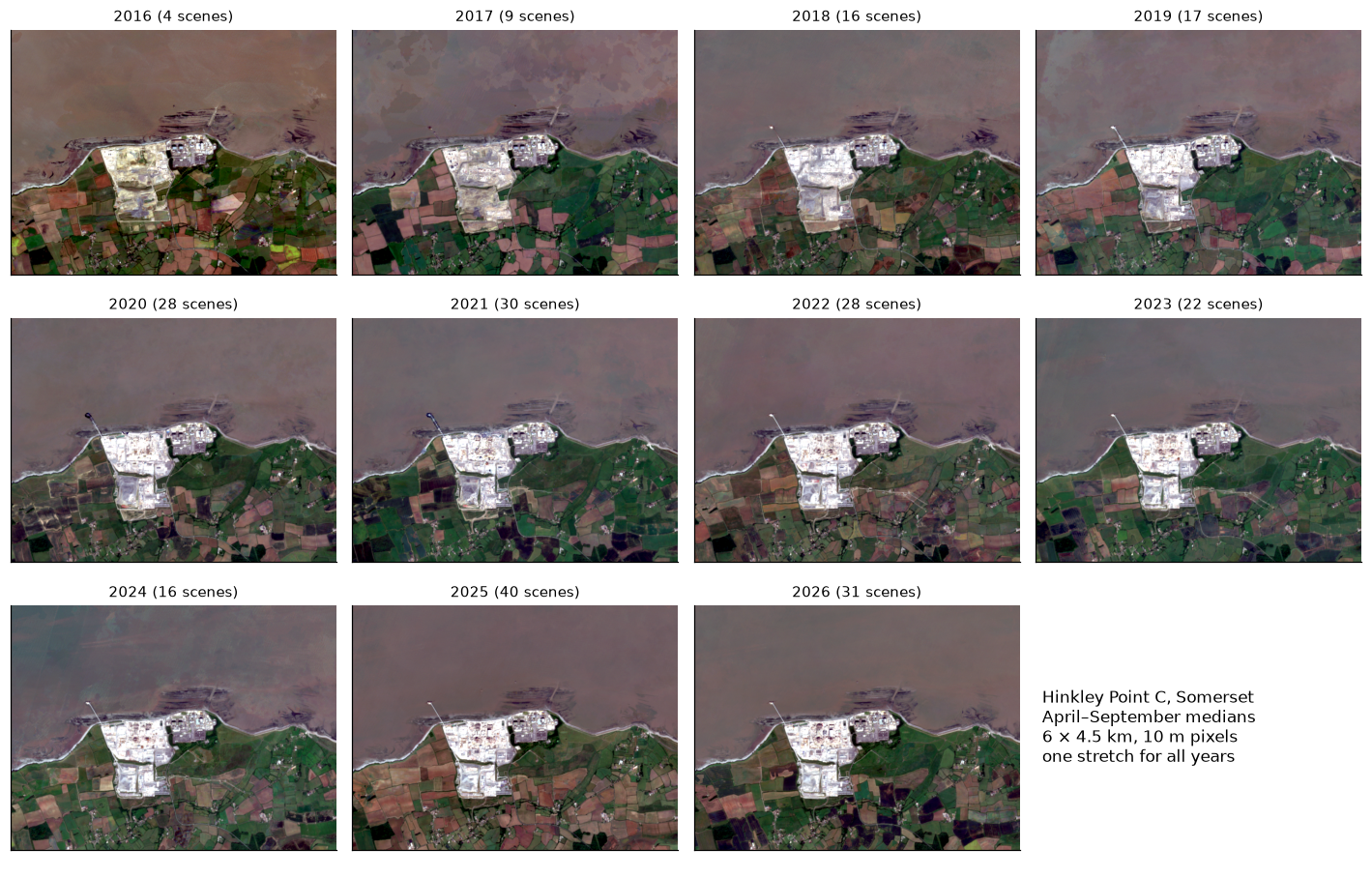
Create a satellite timelapse in Python from free Sentinel-2 imagery. Select clear scenes with STAC, mask cloud, build one median composite per summer, apply a consistent stretch, add date labels and a scale bar, and export an animated GIF, WebP and MP4 of eleven years of construction at Hinkley Point C.
- Level
- Intermediate
- Tested with
- Python 3.12
- Source code
- Download scripts
Key takeaways
- A good timelapse starts with scene selection, not animation. Of 492 April–September Sentinel-2 scenes over Hinkley Point between 2016 and 2026, 241 had at least 40% of the 6 × 4.5 km area clear, measured from each scene's own SCL band. Tile-level cloud cover correlated only −0.58 with the clear fraction of our area.
- A per-pixel median of the SCL-masked scenes for each summer gives one clean frame per year. Every year after 2016 had at least 9 usable scenes; 2016 had 4, because only Sentinel-2A was flying.
- Use one stretch for every frame. Per-frame percentile stretches moved the red high limit between 0.212 and 0.263 reflectance, so the same ground was drawn up to 10 percentage points brighter or darker from year to year: flicker that is not on the ground.
- MP4 and animated WebP are far smaller than GIF. The same 11 frames came to 0.44 MB as WebP and 0.75 MB as a 16-second H.264 MP4 with cross-fades at 800 × 640 px, against 2.44 MB for a GIF cut to 600 × 480 px.
- Inside a 195 ha box around Hinkley Point C, 116 ha (59%) looked different in 2026 from 2016, while bare ground (NDVI below 0.3) stayed at 135–158 ha after 2017: the change is building on an already cleared platform, which a vegetation index alone would miss.
Before you start
- Comfortable with NumPy arrays; the Sentinel-2 Lake Mead tutorial introduces STAC searches and Cloud Optimised GeoTIFFs
- Python 3.10+ with pystac-client, planetary-computer, odc-stac, scipy, pandas, matplotlib, Pillow, imageio and imageio-ffmpeg (which bundles its own ffmpeg)
- An internet connection: Sentinel-2 L2A streams from the Microsoft Planetary Computer with no account or key
Short answer: to make a satellite timelapse in Python, search Sentinel-2 L2A scenes with STAC (the Microsoft Planetary Computer needs no key), keep the scenes that are mostly clear over your area, mask cloud and shadow with the SCL band, take a per-pixel median for each year or season, apply one fixed stretch to every frame, draw the date and a scale bar with Pillow, then write the frames with imageio as a GIF, with Pillow as an animated WebP, and with imageio-ffmpeg as an H.264 MP4. Share the MP4 or WebP: they are three to six times smaller than the GIF.
Satellite timelapses are a good way to show change, and they are easy to get wrong: cloud speckles the frames, the colours flicker from year to year, and a GIF can grow to tens of megabytes. This tutorial builds eleven summer frames of Hinkley Point C, the nuclear power station under construction on the Somerset coast of the Bristol Channel, from 241 Sentinel-2 scenes, and exports a timelapse that weighs less than 1 MB.
You will learn how to:
- find every Sentinel-2 scene of an area for several years with STAC, keeping only the latest processing of each date;
- select scenes by the clear fraction inside your area, measured from the SCL band;
- mask cloud and shadow with SCL plus a small buffer, and correct the 2022 processing offset;
- build one median composite per summer and count clear observations per pixel;
- apply a consistent stretch so that frames are comparable;
- add a date label, scale bar and north arrow with Pillow, and export GIF, WebP and MP4;
- measure the change you are showing, so that the animation is backed by numbers.
All outputs below are real results from timelapse.py, run on 3 November 2026 with Python 3.12, odc-stac 0.5.3, Pillow 13.0.0, imageio 2.38.1 and imageio-ffmpeg 0.8.0 (ffmpeg 9.0.2). The whole script took about a minute.
Why Hinkley Point C?
A timelapse needs a place that changes visibly at 10 m resolution. Hinkley Point C is ideal: a 1.3 × 1.5 km construction site on open farmland, with the older Hinkley Point A and B stations next door as a fixed reference, a jetty built out into the Bristol Channel, and steady work across the whole Sentinel-2 record. The study area is a 6 × 4.5 km rectangle in UTM zone 30N, the native grid of Sentinel-2 tile 30UVB, so nothing needs to be reprojected.
CRS = "EPSG:32630" # UTM 30N, the native grid of tile 30UVBAOI = (487600, 5670700, 493600, 5675200) # 6.0 x 4.5 km: Hinkley Point A, B and C, Stolford, the foreshoreSITE = (489200, 5671650, 490500, 5673150) # 1.3 x 1.5 km box around Hinkley Point C, west of Hinkley Point BTILE = "30UVB"YEARS = list(range(2016, 2027))SEASON = ("04-01", "09-30") # April to SeptemberMIN_CLEAR = 0.4 # keep a scene if at least 40% of the area is clearSCL_BAD = [0, 1, 3, 8, 9, 10] # no data, saturated, cloud shadow, cloud medium/high, cirrusBANDS = ["B02", "B03", "B04", "B08"]We use one frame per summer. April to September gives the most clear days in Britain and avoids the long winter shadows and low sun of a year-round composite. For a place with fast change, such as a reservoir filling, use seasonal or monthly frames instead; the code is the same with a different date grouping.
Step 1: find every candidate scene with STAC
The search uses the area’s bounding box in longitude and latitude, the tile code, and a loose filter on tile cloud cover. Sentinel-2 scenes are sometimes reprocessed, and the Planetary Computer can list both versions, so we keep the latest s2:generation_time for each date and relative orbit:
catalog = pystac_client.Client.open(STAC_URL, modifier=pc.sign_inplace)items = []for y in YEARS: found = catalog.search(collections=["sentinel-2-l2a"], bbox=bbox_ll, datetime=f"{y}-{SEASON[0]}/{y}-{SEASON[1]}", query={"s2:mgrs_tile": {"eq": TILE}, "eo:cloud_cover": {"lt": 80}}).item_collection() # keep the latest processing of each acquisition latest = {} for it in found: k = it.properties["datetime"][:10] + it.id.split("_")[3] # date + relative orbit if k not in latest or it.properties["s2:generation_time"] > latest[k].properties["s2:generation_time"]: latest[k] = it items += list(latest.values())2016: 22 scenes with tile cloud < 80%2017: 28 scenes with tile cloud < 80%2018: 39 scenes with tile cloud < 80%2019: 49 scenes with tile cloud < 80%2020: 56 scenes with tile cloud < 80%2021: 50 scenes with tile cloud < 80%2022: 42 scenes with tile cloud < 80%2023: 37 scenes with tile cloud < 80%2024: 32 scenes with tile cloud < 80%2025: 69 scenes with tile cloud < 80%2026: 68 scenes with tile cloud < 80%492 candidate scenes in total2016 is thin because only Sentinel-2A was in orbit; Sentinel-2B joined in 2017, and Sentinel-2C entered service in 2025 while Sentinel-2A carried on in an extended campaign, which is why 2025 and 2026 have the most scenes.
Step 2: select scenes by the clear fraction of your area
The eo:cloud_cover property describes the whole 110 km tile, not our 27 km² of coast. A much better filter is to read the SCL band of every candidate over the area itself. At 20 m this is only 300 × 225 pixels per scene, so odc.stac.load reads all 492 scenes in seconds:
gb20 = GeoBox.from_bbox(AOI, crs=CRS, resolution=20)scl = odc.stac.load(items, bands=["SCL"], geobox=gb20, resampling="nearest", pool=16)["SCL"]scl_np = scl.valueshas_data = (scl_np != 0).mean(axis=(1, 2))clear = (~np.isin(scl_np, SCL_BAD)).mean(axis=(1, 2))scenes["keep"] = (scenes["coverage"] > 0.99) & (scenes["clear"] >= MIN_CLEAR)read SCL for 492 scenes on a 300 x 225 grid in 4 s candidates kept median_clearyear2016 22 4 17%2017 28 9 41%2018 39 16 77%2019 49 17 73%2020 56 28 77%2021 50 30 70%2022 42 28 72%2023 37 22 60%2024 32 16 41%2025 69 40 56%2026 68 31 82%kept 241 of 492 scenes; correlation of tile cloud with area clear fraction: -0.58The first run took about 30 seconds to read the SCL bands; the 4 s above is a rerun with GDAL’s cache warm. The coverage test (more than 99% of pixels with data) drops scenes at the edge of an orbit’s swath, where the area is only partly imaged.
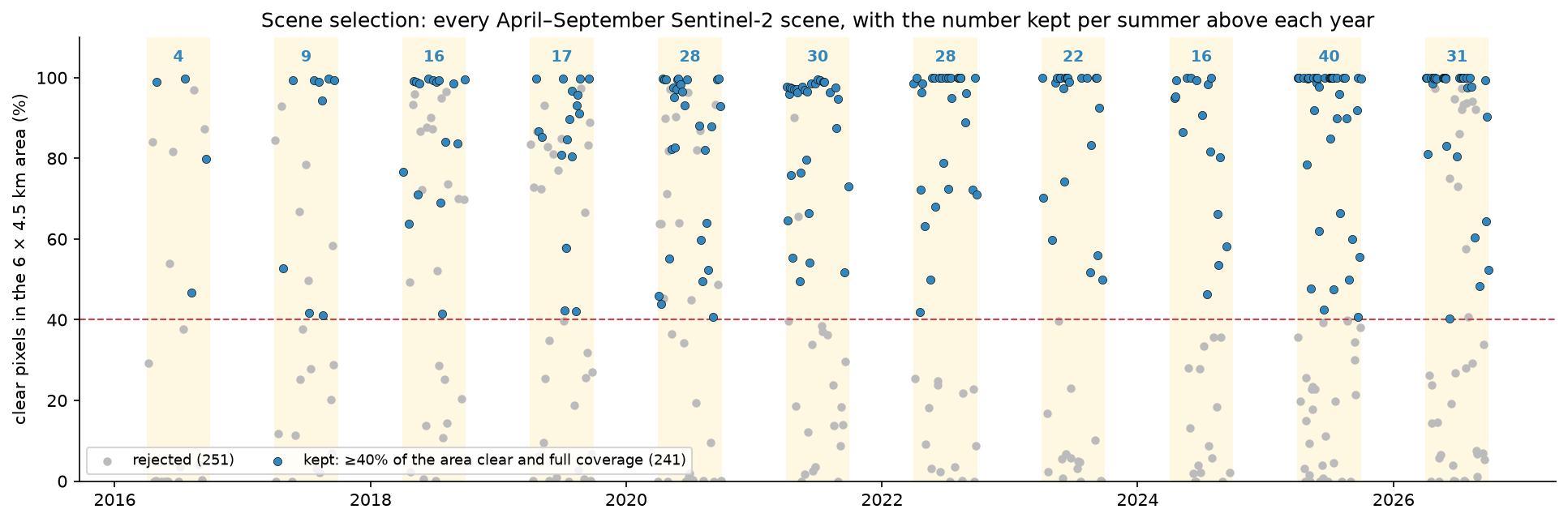
A threshold of 40% clear may seem low, but the median in Step 4 only uses the clear pixels of each scene. A half-clear scene still adds an observation to half the area, which matters most in a thin year like 2016.
Step 3: load the clear scenes and mask cloud and shadow
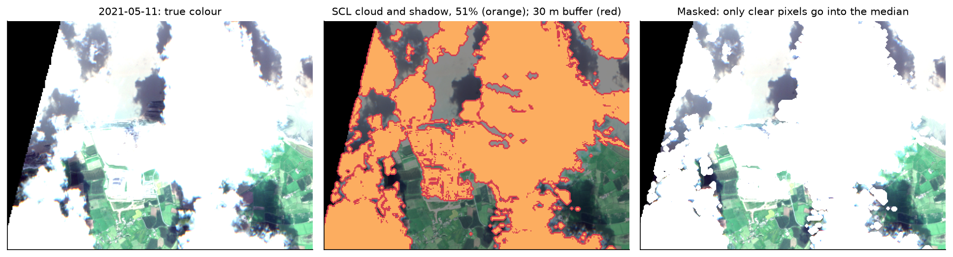
We load blue, green, red, near-infrared and SCL at 10 m for the 241 kept scenes, then turn digital numbers into reflectance. Scenes processed with baseline 04.00 or later (from 25 January 2022, and all reprocessed scenes) carry an offset of 1000; forgetting it makes every frame from 2022 onwards look brighter.
gb10 = GeoBox.from_bbox(AOI, crs=CRS, resolution=10)ds = odc.stac.load(keep_items, bands=BANDS + ["SCL"], geobox=gb10,                   resampling={"SCL": "nearest", "*": "bilinear"}, pool=16)
# Processing baseline 04.00 (25 January 2022) added an offset of 1000 to every DN.offset = np.array([1000 if float(b) >= 4.0 else 0 for b in scenes.loc[scenes["keep"], "baseline"]], dtype="float32")refl = {}for b in BANDS: dn = ds[b].values.astype("float32") refl[b] = np.where(dn == 0, np.nan, (dn - offset[:, None, None]) / 10000)bad = np.isin(ds["SCL"].values, SCL_BAD)bad_buf = np.stack([ndimage.binary_dilation(m, iterations=3) for m in bad]) # 30 m buffer catches hazy cloud edgesfor b in BANDS: refl[b][bad_buf] = np.nanloaded 241 scenes x 5 bands on a 600 x 450 grid in 23 sbaselines: 02.12 (75), 03.00 (29), 04.00 (8), 05.09 (5), 05.10 (47), 05.11 (46), 05.12 (28), 05.13 (3)SCL masks 13.8% of kept pixels; with a 30 m buffer 16.7%Read the processing baseline from each item (s2:processing_baseline) rather than from the date: some older acquisitions on the Planetary Computer have been reprocessed with a newer baseline, and those carry the offset too.
Step 4: one median composite per summer
For each year, np.nanmedian over the time axis ignores masked pixels, so each output pixel is the median of that pixel’s clear observations. We also count those observations, because a median of one or two values is not much better than a single scene:
for y in YEARS: sel = years == y with np.errstate(all="ignore"): comp[y] = {b: np.nanmedian(refl[b][sel], axis=0) for b in BANDS} nclear[y] = np.isfinite(refl["B04"][sel]).sum(axis=0) gap = nclear[y] == 0 # Pixels that were never clear (bright concrete and the sea wall, which SCL often calls cloud, or # persistent cloud) fall back to the median of the unmasked scenes so the frame has no holes. if gap.any(): for b in BANDS: dn = ds[b].values[sel].astype("float32") unmasked = np.where(dn == 0, np.nan, (dn - offset[sel][:, None, None]) / 10000) with np.errstate(all="ignore"): comp[y][b][gap] = np.nanmedian(unmasked[:, gap], axis=0)2016: 4 scenes; clear observations per pixel min 0, median 3; never clear 0.36% (filled from unmasked scenes)2017: 9 scenes; clear observations per pixel min 0, median 7; never clear 0.07% (filled from unmasked scenes)2018: 16 scenes; clear observations per pixel min 0, median 13; never clear 0.06% (filled from unmasked scenes)2019: 17 scenes; clear observations per pixel min 0, median 14; never clear 0.31% (filled from unmasked scenes)2020: 28 scenes; clear observations per pixel min 0, median 22; never clear 0.20% (filled from unmasked scenes)2021: 30 scenes; clear observations per pixel min 0, median 25; never clear 0.09% (filled from unmasked scenes)2022: 28 scenes; clear observations per pixel min 14, median 24; never clear 0.00% (filled from unmasked scenes)2023: 22 scenes; clear observations per pixel min 6, median 19; never clear 0.00% (filled from unmasked scenes)2024: 16 scenes; clear observations per pixel min 3, median 13; never clear 0.00% (filled from unmasked scenes)2025: 40 scenes; clear observations per pixel min 18, median 34; never clear 0.00% (filled from unmasked scenes)2026: 31 scenes; clear observations per pixel min 16, median 27; never clear 0.00% (filled from unmasked scenes)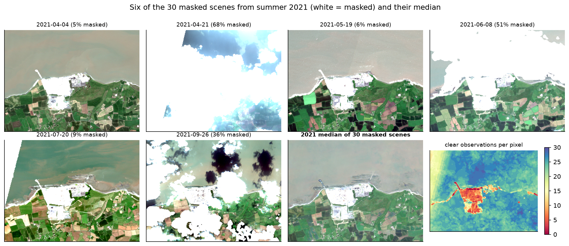
The clear-observation map explains the fallback in the code. Before 2022 a few pixels, mostly on the jetty, the sea wall and the brightest parts of the site, were never clear in SCL, because Sen2Cor confuses bright artificial surfaces with cloud. Leaving them as holes put black dots on the frames, so they take the median of the unmasked scenes instead. That is never more than 0.36% of a frame.
Step 5: one stretch for every frame
Reflectance must be stretched to 0–255 for display. The usual approach for one image, a 1st–99th percentile stretch, is wrong for a timelapse when applied to each frame separately: each year’s limits depend on how much bright concrete, dark sea or ripe crop happens to be in the picture, so the same surface is drawn differently from frame to frame. We compute the limits once from all eleven composites together:
pool = np.stack([np.stack([comp[y][b] for b in ["B04", "B03", "B02"]], axis=-1) for y in YEARS])LO = np.nanpercentile(pool, 1, axis=(0, 1, 2))HI = np.nanpercentile(pool, 99, axis=(0, 1, 2))GAMMA = 1.4

def rgb(r, g, b, lo, hi, gamma=1.0):    """Linear stretch between lo and hi (per band), then gamma; returns floats in 0..1."""    x = np.dstack([r, g, b])    x = np.clip((x - lo) / (hi - lo), 0, 1) ** (1 / gamma)    return np.nan_to_num(x, nan=0.0)

frames_global = {y: rgb(comp[y]["B04"], comp[y]["B03"], comp[y]["B02"], LO, HI, GAMMA) for y in YEARS}global stretch (reflectance) R/G/B low 0.029 / 0.048 / 0.024, high 0.248 / 0.222 / 0.198, gamma 1.4per-frame red limits move between years: high 0.212-0.263, low 0.023-0.033 (the global stretch fixes them at 0.248 and 0.029)a red reflectance of 0.1 is drawn at 0.42-0.52 of full brightness with per-frame stretches, and at 0.45 in every frame with one stretch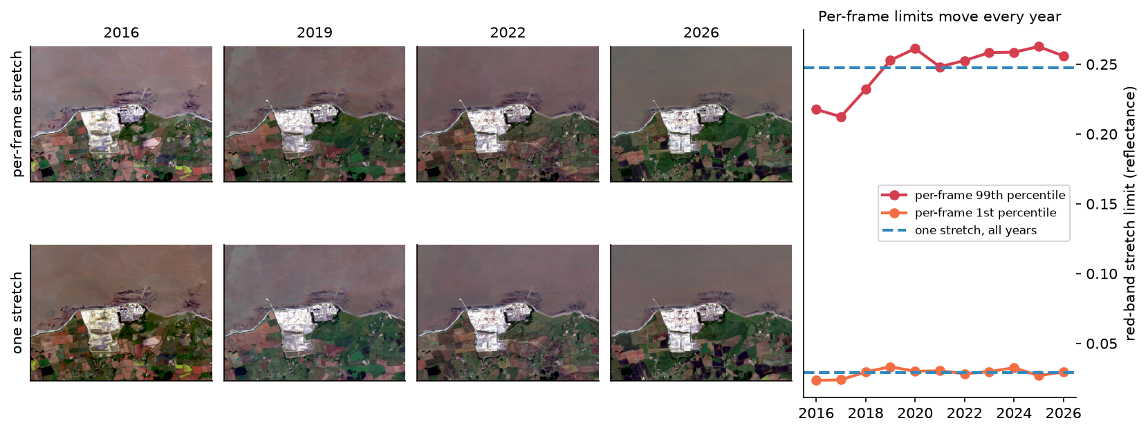
The gamma of 1.4 lifts the dark green fields and the muddy water of the Bristol Channel without burning out the concrete. If your scene has snow or cloud-free desert, use a higher upper percentile so that the brightest surface is not clipped.
Step 6: add labels, a scale bar and export GIF, WebP and MP4
Each frame is drawn with Pillow at 800 × 600 pixels (the 600 × 450 composite scaled by 4/3), plus a 40-pixel caption strip, making 800 × 640. Both dimensions are multiples of 16, so the H.264 encoder does not have to pad the video. The year label sits in a dark box in the top-left corner; a 1 km scale bar is 100 composite pixels times the display scale:
SCALE = 4 / 3                                       # 600 x 450 px -> 800 x 600 pxW, H = int(gb10.shape[1] * SCALE), int(gb10.shape[0] * SCALE)BAR = 40                                            # caption strip; 600 + 40 px is a multiple of 16 for H.264

def make_frame(y):    img = Image.fromarray((frames_global[y] * 255).round().astype("uint8")).resize((W, H), Image.Resampling.LANCZOS)    canvas = Image.new("RGB", (W, H + BAR), (20, 22, 28))    canvas.paste(img, (0, 0))    d = ImageDraw.Draw(canvas)    # date label: a dark box in the top-left corner    d.rounded_rectangle((14, 14, 124, 60), radius=6, fill=(20, 22, 28))    d.text((24, 18), str(y), font=f_year, fill=(255, 255, 255))    # scale bar: 1 km = 100 px at 10 m, times the display scale    px_km = 1000 / 10 * SCALE    x0, y0 = W - 24 - px_km, H - 34    d.rounded_rectangle((x0 - 12, y0 - 26, x0 + px_km + 12, y0 + 18), radius=6, fill=(20, 22, 28))    d.rectangle((x0, y0, x0 + px_km / 2, y0 + 8), fill=(255, 255, 255))    d.rectangle((x0 + px_km / 2, y0, x0 + px_km, y0 + 8), fill=(20, 22, 28), outline=(255, 255, 255), width=2)    d.text((x0, y0 - 22), "0", font=f_scale, fill=(255, 255, 255))    d.text((x0 + px_km - 30, y0 - 22), "1 km", font=f_scale, fill=(255, 255, 255))    # north arrow    d.polygon([(W - 34, 20), (W - 44, 46), (W - 24, 46)], fill=(255, 255, 255))    d.text((W - 40, 48), "N", font=f_scale, fill=(255, 255, 255))    # caption strip    d.text((14, H + 3), f"Hinkley Point C, Somerset · Sentinel-2 median, April–September {y} ({n_kept[y]} clear scenes)",           font=f_small, fill=(255, 255, 255))    d.text((14, H + 21), "Contains modified Copernicus Sentinel data 2016–2026 · technicalgis.com",           font=f_small, fill=(190, 190, 190))    return np.asarray(canvas)

frames = [make_frame(y) for y in YEARS]
A scale bar is only true when the image is in a projected CRS with square pixels, as it is here (UTM, 10 m). On a Web Mercator basemap the scale changes with latitude; at 51° north it is about 1.6 times too large.
Exporting needs three different tools. imageio writes the GIF, Pillow writes the animated WebP, and imageio-ffmpeg, which ships its own ffmpeg binary, writes the MP4. For the video we hold each year for one second at 12 frames per second and add a five-frame cross-fade between years:
DUR = [1100] * (len(frames) - 1) + [2200]           # ms per frame; hold the last year longer
# The GIF is 600 px wide: 256 colours per frame and LZW compression make GIFs several times larger than WebP or MP4.gif_frames = [np.asarray(Image.fromarray(f).resize((600, 480), Image.Resampling.LANCZOS)) for f in frames]iio.imwrite(OUT / "hinkley_timelapse.gif", gif_frames, duration=DUR, loop=0)pil_frames = [Image.fromarray(f) for f in frames]pil_frames[0].save(OUT / "hinkley_timelapse.webp", save_all=True, append_images=pil_frames[1:], duration=DUR,                   loop=0, quality=80, method=6)
# MP4: 12 frames per second with a short cross-fade between years, H.264 in yuv420p so every browser plays it.FPS, HOLD, FADE = 12, 12, 5video = []for i, f in enumerate(frames): video += [f] * (HOLD if i < len(frames) - 1 else HOLD * 2) if i < len(frames) - 1: a, b = f.astype("float32"), frames[i + 1].astype("float32") video += [((1 - t) * a + t * b).round().astype("uint8") for t in np.linspace(0, 1, FADE + 2)[1:-1]]writer = imageio_ffmpeg.write_frames(str(OUT / "hinkley_timelapse.mp4"), (W, H + BAR), fps=FPS, codec="libx264", pix_fmt_out="yuv420p", quality=None, output_params=["-crf", "26", "-preset", "slow", "-movflags", "+faststart"])writer.send(None)for f in video: writer.send(np.ascontiguousarray(f))writer.close()11 frames of 800 x 640 pxGIF 2.44 MB (11 frames at 600 x 480 px, 256 colours per frame)WebP 0.44 MB (lossy, quality 80)MP4 0.75 MB (194 frames at 12 fps, 16.2 s, H.264 CRF 26)poster PNG 0.66 MBAt the full 800 × 640 pixels the GIF was 3.9 MB, nine times the WebP, even though it carries no cross-fades. GIF stores each frame with its own 256-colour palette and lossless compression, which suits flat graphics but not satellite imagery. Use the MP4 for websites and slides, the WebP where a video tag is awkward, and the GIF only where nothing else is accepted, such as some chat and email clients. The +faststart flag moves the MP4’s index to the front of the file so that browsers can start playing before the download finishes, and yuv420p is the pixel format that every browser supports.
Step 7: measure what the timelapse shows
An animation persuades, but it is worth checking with numbers. We take a 195 ha box around Hinkley Point C (keeping out Hinkley Point B) and measure two things each year: the area whose visible colour differs from 2016 by more than 0.05 in reflectance (Euclidean distance over red, green and blue), and the area of bare ground, with NDVI below 0.3.
ndvi = {y: (comp[y]["B08"] - comp[y]["B04"]) / (comp[y]["B08"] + comp[y]["B04"]) for y in YEARS}diff = {y: np.sqrt(sum((comp[y][b] - comp[YEARS[0]][b]) ** 2 for b in RGB)) for y in YEARS}CHANGE = 0.05 # visible-band reflectance distance that counts as changedfor y in YEARS: rows.append({"year": y, "changed_since_2016_ha": float((diff[y][r0:r1, c0:c1] > CHANGE).sum() * 0.01), "unvegetated_ha": float((ndvi[y][r0:r1, c0:c1] < 0.3).sum() * 0.01), "site_mean_ndvi": float(np.nanmean(ndvi[y][r0:r1, c0:c1]))}) year changed_since_2016_ha unvegetated_ha site_mean_ndvi 2016 0 116 0.25 2017 92 158 0.16 2018 98 145 0.17 2019 98 141 0.19 2020 106 138 0.21 2021 105 136 0.22 2022 113 137 0.20 2023 123 141 0.21 2024 120 138 0.23 2025 118 136 0.21 2026 116 135 0.24site box 195 ha; changed since 2016: 116 ha by 2026 (59%); unvegetated share 60%-81% in every year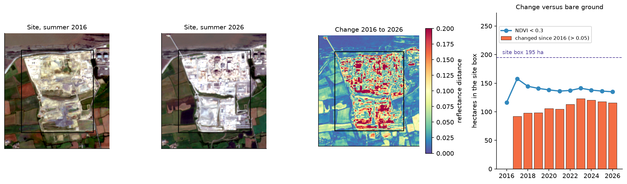
The two measures tell different stories, and both are true. The site was levelled during preparatory works before Sentinel-2 began, so a vegetation index sees bare ground throughout. What the timelapse shows, and the colour-difference measure picks up, is building. If you use a timelapse to report change, pick a measure that matches the change.
Pitfalls and limitations
- One clear scene is not a composite. 2016 has only four kept scenes and a median of three clear observations per pixel, so its frame is noisier and its colours less reliable than later years. Mention thin years in any caption, or drop them.
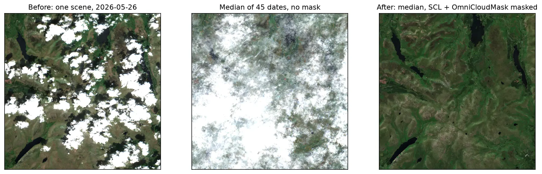
- SCL calls bright concrete cloud. Over the site and the jetty, many clear-sky pixels were masked. We filled never-clear pixels from the unmasked median, which brings back any real cloud at those pixels too. A better mask, such as OmniCloudMask from our cloud masking tutorial, reduces the problem.
- Medians blur fast change. A summer median shows the typical state between April and September. A building finished in August may not appear until the next year’s frame. For month-by-month change use shorter windows and accept more cloud.
- Crops change colour every year. The farmland flickers between green, brown and pink because crops rotate and harvest dates vary. That is real, not a processing error, but it distracts from the site. A greyscale or desaturated background, or a mask around the area of interest, can help.
- Tide and sea state vary. The intertidal mud of Bridgwater Bay is exposed in some scenes and covered in others; the median smooths it, but the shoreline is not a fixed line between frames.
- Different satellites, small differences. Sentinel-2A, 2B and 2C have slightly different spectral responses, and the three-satellite mix changes over the record. For a display timelapse this is invisible; for quantitative change detection, harmonise first.
- Respect the licence in the frame. Copernicus Sentinel data are free, but the attribution “Contains modified Copernicus Sentinel data [year]” should appear, which is why it is burnt into every frame.
Frequently asked questions
How do I make a satellite timelapse in Python?
Find the scenes with STAC (for example, pystac_client on the Microsoft Planetary Computer), load them with odc.stac.load on a fixed grid, mask cloud, take a median for each period, apply one stretch to every frame, label the frames with Pillow and write them with imageio (GIF), Pillow (WebP) or imageio-ffmpeg (MP4). The script in this tutorial does all of that in about 430 lines and a minute of run time.
How do I make a satellite timelapse GIF smaller?
Reduce the pixel size first, because GIF size scales with area: our GIF went from 3.9 MB at 800 × 640 to 2.44 MB at 600 × 480. Fewer frames and fewer colours also help. But the biggest saving is not to use GIF at all: the same animation was 0.44 MB as an animated WebP and 0.75 MB as an MP4 with cross-fades, and both look better.
Why do the colours flicker in my timelapse?
Usually because each frame has its own stretch. A per-frame percentile stretch adapts to whatever is brightest in that frame, so the same ground is drawn brighter or darker from year to year. Compute the stretch limits once, from all frames together, and apply them to every frame. Remaining flicker is usually real, such as crops, tides or seasonal vegetation.
Can I make a timelapse with Landsat instead of Sentinel-2?
Yes. Landsat goes back to the 1980s, at 30 m. Load landsat-c2-l2 from the Planetary Computer, mask with the qa_pixel band instead of SCL, and apply the Collection 2 scale factor (reflectance = DN × 0.0000275 − 0.2). Landsat 7 images after 2003 have stripes of missing data, which a median of several scenes fills.
How do I embed a satellite timelapse in a web page?
Use an MP4 in a <video> element with muted, loop and playsinline and a poster image, as on this page. Encode it with H.264 in yuv420p and +faststart, and keep both dimensions multiples of 16. An animated WebP in an <img> tag is the next best choice; a GIF should be the last resort.
Does Google Earth Engine do this more easily?
Earth Engine has built-in timelapse helpers, and the geemap package can make a GIF in a few lines. It needs an account, and the processing happens on Google’s servers. The approach here runs anywhere with open data and gives you full control over scene selection, masking and the stretch.
Next steps
- Improve the mask: Sentinel-2 cloud and shadow masking in Python compares SCL with s2cloudless and OmniCloudMask.
- Turn the frames into a chart: NDVI time series in Python with Sentinel-2 and odc-stac follows the same STAC and odc-stac pattern for a per-date index.
- Measure a moving coastline: coastal erosion and shoreline change with Sentinel-2 extracts shorelines from the same kind of composites.
- Map forest loss year by year: deforestation detection in Python is another change story that animates well.
- Scale up: parallel raster processing in Python with dask and rioxarray builds a median composite over a whole 110 km Sentinel-2 tile without running out of memory.
- Make print-quality maps of single frames: maps in Python with matplotlib and Cartopy.
Data and licences
- Sentinel-2 L2A: contains modified Copernicus Sentinel data 2016–2026, processed by ESA. Accessed as Cloud Optimised GeoTIFFs from the Microsoft Planetary Computer on 3 November 2026. Copernicus Sentinel data are free and open under the Copernicus data licence; the attribution is burnt into every frame.
- Fonts: DejaVu Sans, bundled with matplotlib (free licence).
- Code:
timelapse.py, tested with Python 3.12.0, pystac-client 0.9.1, planetary-computer 1.0.0, odc-stac 0.5.3, odc-geo 0.5.4, xarray 2026.9.0, NumPy 2.5.4, SciPy 1.18.1, pandas 3.1.0, matplotlib 3.11.2, Pillow 13.0.0, imageio 2.38.1 and imageio-ffmpeg 0.8.0 (ffmpeg 9.0.2).
Key terms
- Timelapse
- A sequence of images of the same place at regular intervals, played quickly so that slow change becomes visible. For satellite data each frame is usually a composite of many scenes rather than a single date.
- Median composite
- An image made by taking, for each pixel and band, the median of all clear observations in a period. It removes remaining cloud, shadow and one-off events such as a passing ship.
- SCL
- Scene Classification Layer: a 20 m band in every Sentinel-2 L2A product that labels each pixel as vegetation, water, cloud, cirrus, cloud shadow and so on. It is used here both to choose scenes and to mask them.
- Display stretch
- The mapping from surface reflectance to screen brightness, usually a linear stretch between a low and high limit followed by a gamma curve. A timelapse needs the same stretch on every frame.
- Processing baseline
- The version of ESA's Sentinel-2 processing chain. Since baseline 04.00 (25 January 2022), L2A digital numbers carry an offset of 1000 that must be removed before comparing older and newer scenes.
- CRF
- Constant Rate Factor: the quality setting of the H.264 video encoder. Lower is better quality and bigger files; 18–28 is the usual range.
Data for this tutorial
- Microsoft Planetary Computer · Sentinel-2 L2A as Cloud Optimised GeoTIFFs via STAC, including the SCL band
- Copernicus Data Space Ecosystem · The official Sentinel-2 archive
Licences and formats for each source are listed in the GIS data sources catalogue.