Parallel raster processing in Python with dask and rioxarray: a whole Sentinel-2 tile without running out of memory

Short answer: to process a satellite raster that is too big for memory in Python, open it with rioxarray.open_rasterio(path, chunks={"band": 1, "x": 2048, "y": 2048}). You get a lazy dask array instead of a NumPy array. Write the calculation with ordinary xarray operations, which builds a task graph, then either call .compute() on a result that fits in memory, or write it straight to disk with .rio.to_raster(path, tiled=True, windowed=True, lock=threading.Lock()). Choose chunks that are whole multiples of the file’s internal tiles and roughly 10–100 MB each, and keep the axis you reduce over (here, time) in one chunk.

A single Sentinel-2 band is 10980 × 10980 pixels: 120 million values, 241 MB as uint16 and 482 MB as float32. Stack a few dates and bands, convert to float for an index, and a plain NumPy script runs out of memory long before it runs out of data. This tutorial takes eight full Sentinel-2 scenes of tile 30UXC (from Oxford and Aylesbury to central London, March to November 2025), computes NDVI for each date and reduces them to a median NDVI map: 1.93 billion input pixels, processed on a laptop-sized memory budget.

You will learn how to:

1. find and download whole Sentinel-2 tiles with STAC, and check how they are stored;
2. open them lazily with rioxarray and choose a chunk size;
3. build the median NDVI as a task graph and see what dask will run;
4. watch a run with dask diagnostics: the task stream, CPU and memory;
5. compare peak memory with the same calculation in eager NumPy;
6. time five chunk sizes and five thread counts, the read lock and a LocalCluster;
7. write the result to disk chunk by chunk as a tiled, compressed GeoTIFF.

All outputs below are real results from dask_raster.py and its helper raster_pipeline.py, run on 3 November 2026 with Python 3.12, dask 2026.8.0, xarray 2026.9.0 and rioxarray 0.23.0 on a Windows 11 workstation with 16 cores (32 threads) and 68 GB of RAM. The whole script took 25 minutes, most of it in the timing grid of Step 6.

Step 1: download eight whole Sentinel-2 scenes

Dask works on remote files too, but benchmarks over the internet mostly measure the network. So the script downloads bands B04 (red) and B08 (near infrared) for eight low-cloud dates once, with a STAC search on the Microsoft Planetary Computer. Where two processings of the same date exist, it keeps the latest:

catalog = pystac_client.Client.open(STAC_URL, modifier=pc.sign_inplace)

def find_item(date):
    items = catalog.search(collections=["sentinel-2-l2a"], datetime=date,
                           query={"s2:mgrs_tile": {"eq": TILE}, "s2:nodata_pixel_percentage": {"lt": 1}}).item_collection()
    return sorted(items, key=lambda i: i.properties["s2:generation_time"])[-1]

jobs = []
for d in DATES:
    it = find_item(d)
    jobs += [(it.assets[b].href, band_path(d, b)) for b in ["B04", "B08"]]
with ThreadPoolExecutor(4) as ex:
    fetched = sum(ex.map(lambda j: download(*j), jobs))

2025-03-06  S2B_MSIL2A_20250306T110829_R137_T30UXC_20250306T133711  tile cloud 3.7%  no data 0.0002%
2025-04-02  S2A_MSIL2A_20250402T110651_R137_T30UXC_20250402T201716  tile cloud 1.0%  no data 0.0001%
2025-04-05  S2B_MSIL2A_20250405T110619_R137_T30UXC_20250405T132414  tile cloud 0.3%  no data 0.0000%
2025-04-30  S2C_MSIL2A_20250430T110641_R137_T30UXC_20250430T151423  tile cloud 6.5%  no data 0.0000%
2025-05-02  S2A_MSIL2A_20250502T110701_R137_T30UXC_20250502T181413  tile cloud 2.1%  no data 0.0000%
2025-06-19  S2C_MSIL2A_20250619T110641_R137_T30UXC_20250619T151116  tile cloud 0.2%  no data 0.0000%
2025-07-11  S2A_MSIL2A_20250711T110651_R137_T30UXC_20250711T153113  tile cloud 5.2%  no data 0.0000%
2025-11-21  S2B_MSIL2A_20251121T111259_R137_T30UXC_20251121T120801  tile cloud 4.9%  no data 0.0005%
16 files on disk, 4.58 GB compressed
each file: 10980 x 10980 px, uint16, deflate, internal tiles (512, 512), overviews [2, 4, 8, 16]
uncompressed: 8 dates x 2 bands x 10980 x 10980 uint16 = 3.86 GB (7.72 GB as float32)

All eight dates come from relative orbit 137, which covers the whole tile, and all three Sentinel-2 satellites (2A, 2B and 2C) contribute. The line that matters most for dask is internal tiles (512, 512): the file is stored in 512 × 512 blocks, and any read touches whole blocks.

We chose clear dates on purpose, so that the tutorial is about dask rather than cloud. For a real composite you would mask cloud first; see Sentinel-2 cloud and shadow masking in Python.

Step 2: open lazily and choose a chunk size

rioxarray.open_rasterio with a chunks= argument returns a dask-backed DataArray. It reads the file headers, not the pixels. We open each band of each date with the same chunks and concatenate them along a new time dimension:

def open_stack(dates, chunk, lock=False):
    chunks = {"band": 1, "y": chunk, "x": chunk}
    red, nir = [], []
    for d in dates:
        red.append(rioxarray.open_rasterio(band_path(d, "B04"), chunks=chunks, lock=lock).squeeze("band", drop=True))
        nir.append(rioxarray.open_rasterio(band_path(d, "B08"), chunks=chunks, lock=lock).squeeze("band", drop=True))
    time_index = xr.Variable("time", np.array(dates, dtype="datetime64[ns]"))
    return xr.concat(red, dim=time_index), xr.concat(nir, dim=time_index)

The lock argument matters more than it looks. rioxarray’s default puts one shared lock around all reads; we pass lock=False so that every thread can read and decompress at the same time. Step 6 measures the difference.

opened 16 files in 0.10 s without reading any pixels
<xarray.DataArray (time: 8, y: 10980, x: 10980)> Size: 2GB
dask.array<concatenate, shape=(8, 10980, 10980), dtype=uint16, chunksize=(1, 2048, 2048), chunktype=numpy.ndarray>

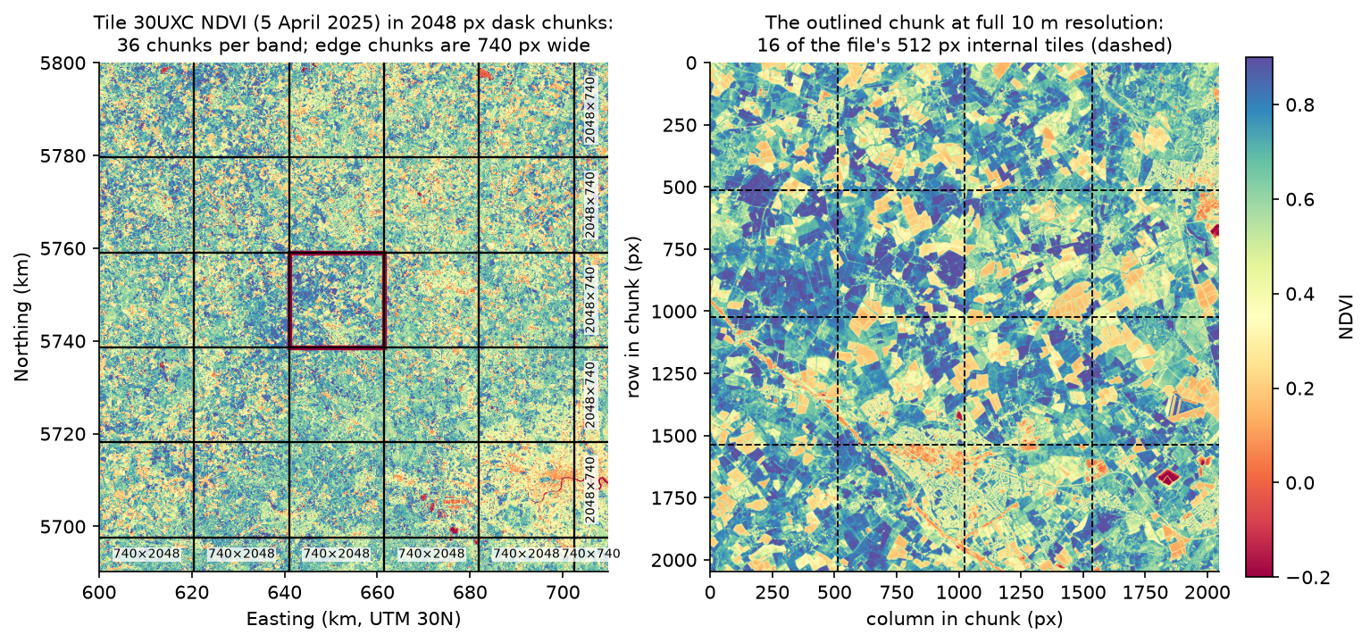
chunk size options for a 10980 x 10980 band:
   256 px:  1849 chunks per band,   0.3 MB per float32 chunk,     2 MB per 8-date block for the median
   512 px:   484 chunks per band,   1.0 MB per float32 chunk,     8 MB per 8-date block for the median
  1024 px:   121 chunks per band,   4.2 MB per float32 chunk,    34 MB per 8-date block for the median
  2048 px:    36 chunks per band,  16.8 MB per float32 chunk,   134 MB per 8-date block for the median
  4096 px:     9 chunks per band,  67.1 MB per float32 chunk,   537 MB per 8-date block for the median

Three rules decide the chunk size:

• Align with the file’s blocks. All five options are multiples of 512, so no chunk splits an internal tile. A 1000 px chunk would make neighbouring chunks decompress the same tiles twice.
• Aim for roughly 10–100 MB per chunk of the working data type. Smaller chunks mean more tasks, and each task costs the scheduler a few hundred microseconds whatever its size. Larger chunks mean fewer opportunities to run in parallel, and more memory per thread.
• Think about the reduction. A median needs every date of a pixel in one place, so the whole time axis goes into one chunk (time: -1 in Step 3). With 2048 px chunks, one 8-date float32 block is 134 MB; with 4096 px it is 537 MB per thread, which adds up quickly with 16 threads.

Step 3: build the median NDVI as a task graph

The calculation is ordinary xarray. Sentinel-2 L2A data processed with baseline 04.00 or later carry an offset of 1000 on every digital number, and 0 means no data:

OFFSET = 1000          # processing baseline 04.00+ adds 1000 to every DN

def median_ndvi(red, nir):
    red = red.where(red > 0).astype("float32") - OFFSET          # DN 0 is no data
    nir = nir.where(nir > 0).astype("float32") - OFFSET
    ndvi = (nir - red) / (nir + red)
    ndvi = ndvi.where(np.isfinite(ndvi))
    ndvi = ndvi.chunk({"time": -1})                              # a median needs every date in one chunk
    out = ndvi.median("time", skipna=True).astype("float32")
    out.attrs = {}                                               # drop the uint16 _FillValue/scale attributes
    return out

Calling median_ndvi returns instantly. The result is still a dask array, and its graph tells us how much work dask has planned:

<xarray.DataArray (y: 10980, x: 10980)> Size: 482MB
dask.array<nanmedian, shape=(10980, 10980), dtype=float32, chunksize=(2048, 2048), chunktype=numpy.ndarray>

2048 px chunks: 6136 tasks in 81 layers; output 482 MB in 36 chunks
   256 px chunks: 314346 tasks, 1849 output chunks
   512 px chunks:  82296 tasks,  484 output chunks
  1024 px chunks:  20586 tasks,  121 output chunks
  2048 px chunks:   6136 tasks,   36 output chunks
  4096 px chunks:   1546 tasks,    9 output chunks
two dates in 2 x 2 chunks: 180 tasks as written, 52 after dask fuses chains of element-wise steps
graph as written: 180 tasks, 228 dependencies, 14 tasks on the longest path
task types: concatenate 16, elementwise 104, median 4, open file 4, read chunk 48, rechunk 4

The number of tasks grows with the square of the chunk count: halving the chunk size from 512 to 256 px quadruples the graph to over 300,000 tasks. Before running anything, dask optimises the graph, fusing chains of element-wise steps (mask, subtract, divide) into single tasks; for the full 2048 px graph that took 6,136 tasks down to 1,513.

The full graph is too big to draw, but the same pipeline on two dates and 2 × 2 chunks is small enough. You can draw your own with med.data.visualize() (it needs Graphviz), or with networkx as the script does:

small = median_ndvi(*open_stack(DATES[:2], 5490))
dsk = dict(small.data.__dask_graph__())
G = nx.DiGraph()
for k in dsk:
    G.add_node(k)
    G.add_edges_from((dep, k) for dep in get_dependencies(dsk, k) if dep in dsk)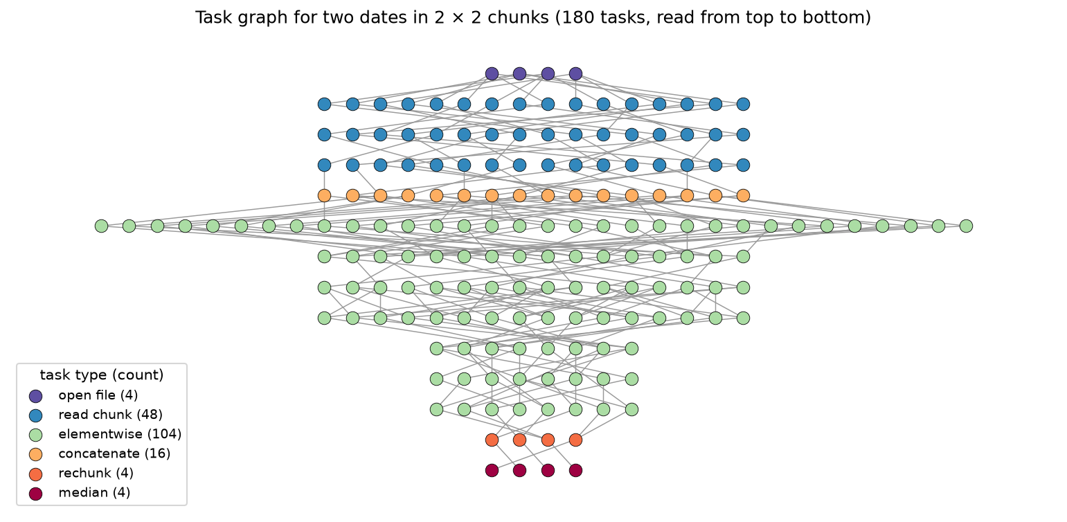

The shape of the graph is the key to why dask saves memory: each output chunk depends only on its own column of inputs. Dask can read one column, reduce it and release the inputs before it reads the next, so only a few columns need to be in memory at once.

Step 4: watch the run with dask diagnostics

Nothing has been read yet. compute() runs the graph on the threaded scheduler. Two context managers record what happens: dask’s own Profiler logs the start and end of every task on every thread, and a small psutil sampler from raster_pipeline.py records the process memory and CPU every 0.1 s:

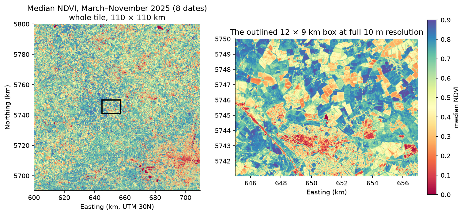
with dask.config.set(scheduler="threads", num_workers=8):
    with Profiler() as prof, RSSSampler(interval=0.1) as rprof, ProgressBar(dt=10, out=sys.stdout):
        result = med.compute()

[                                        ] | 0% Completed | 294.90 us
[#######################                 ] | 59% Completed | 10.01 s
[########################################] | 100% Completed | 20.01 s
computed in 20.1 s: 1513 tasks; process memory 0.35 GB at start, 6.64 GB at peak; mean CPU 694% (800% = 8 busy threads)
median NDVI: mean 0.584; 100.00% of pixels valid; 6,874 km² above 0.6 and 192 km² below 0.1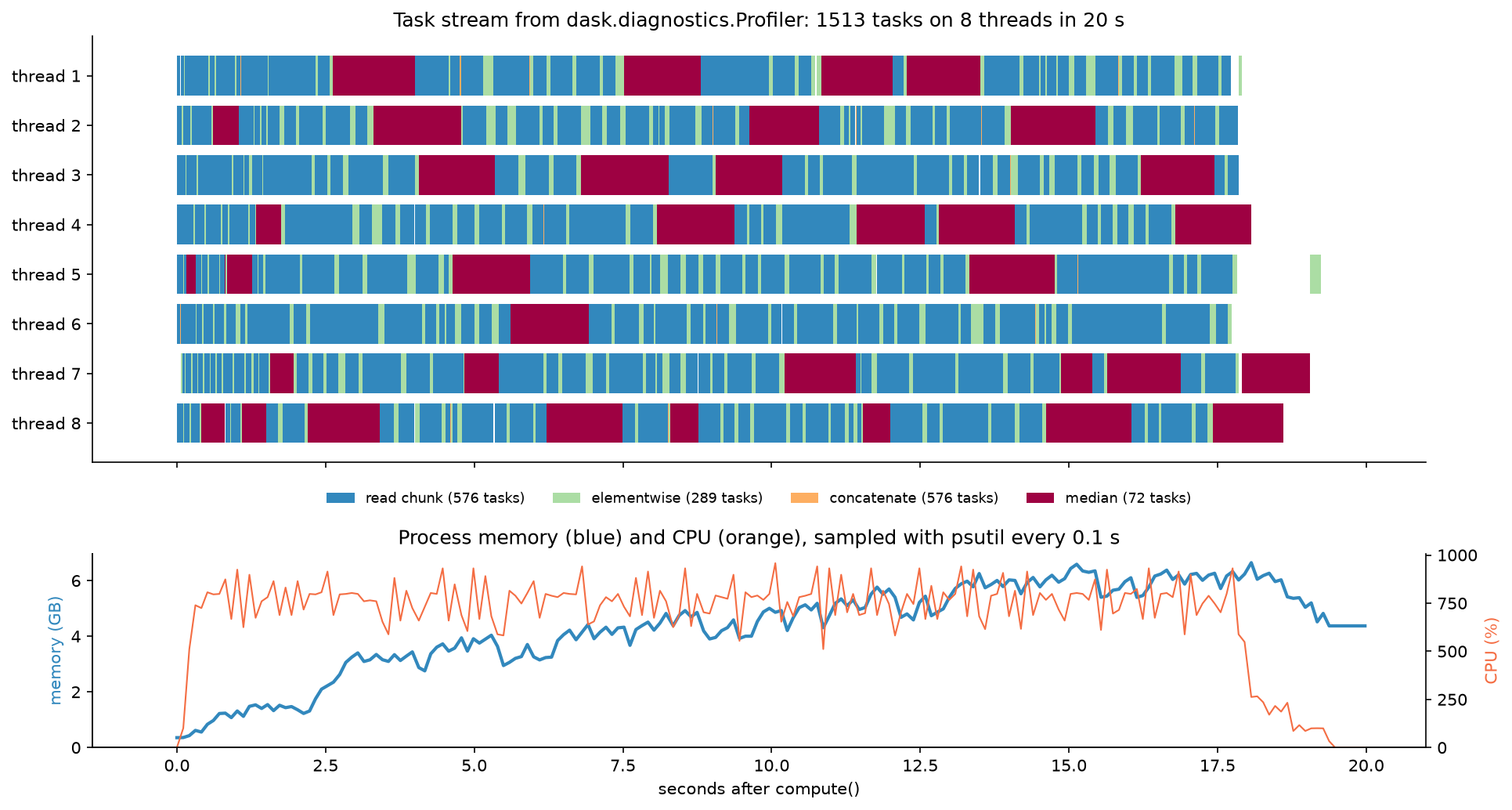

The diagnostics answer the two questions that matter for any dask job:

• Are all the threads busy? Yes. The task stream has almost no gaps, and the mean CPU was 694% of the 800% available. Gaps in the stream would mean that tasks are waiting on each other, on a lock or on the disk.
• Where does the memory go? The working set is a few chunks per thread. The memory line rises steadily because the result itself (482 MB of float32) is assembled in memory, and because the operating system does not hand memory back immediately; the peak of 6.6 GB is well under the 7.7 GB the float32 inputs alone would need.

The computed median is a reasonable picture of southern England in 2025: mean NDVI 0.58, with 6,874 km² of the 12,056 km² tile above 0.6 (crops and grass in leaf) and 192 km² below 0.1 (water, roofs and roads).

Step 5: peak memory, eager NumPy against dask

To see what dask saves, raster_pipeline.py also does the calculation the eager way: read every band into a NumPy array, stack them, and call np.nanmedian. Each run starts in a fresh Python process and records the peak memory above that process’s starting point:

def eager_median_ndvi(dates):
    def read(d, b):
        with rasterio.open(band_path(d, b)) as src:
            return src.read(1)

    red = np.stack([read(d, "B04") for d in dates]).astype("float32")
    nir = np.stack([read(d, "B08") for d in dates]).astype("float32")
    red[red == 0] = np.nan
    nir[nir == 0] = np.nan
    red -= OFFSET
    nir -= OFFSET
    ndvi = (nir - red) / (nir + red)
    del red, nir
    ndvi[~np.isfinite(ndvi)] = np.nan
    return np.nanmedian(ndvi, axis=0).astype("float32")

eager NumPy, 1 date(s):   18.9 s, peak  8.95 GB  (mean NDVI 0.4903)
eager NumPy, 2 date(s):   35.3 s, peak  9.92 GB  (mean NDVI 0.5125)
eager NumPy, 4 date(s):   62.9 s, peak 12.37 GB  (mean NDVI 0.5475)
dask,        1 date(s):    3.9 s, peak  2.12 GB  (mean NDVI 0.4903)
dask,        2 date(s):    6.1 s, peak  2.50 GB  (mean NDVI 0.5125)
dask,        4 date(s):   10.4 s, peak  4.12 GB  (mean NDVI 0.5475)
dask,        8 date(s):   19.0 s, peak  6.36 GB  (mean NDVI 0.5836)
eager peak grows by 1.15 GB per date: about 17 GB for 8 dates and 88 GB for the 70 or so scenes a year of this tile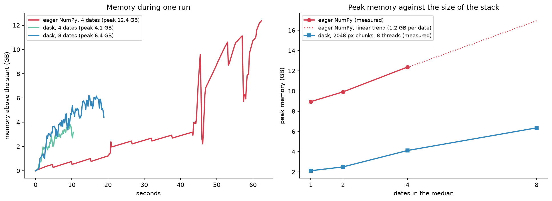

Three things stand out:

• The results agree. The mean NDVI matches to four decimal places for every stack size, so dask changes how the work is scheduled, not what is computed.
• Eager NumPy is greedy even for one date. Reading a single date (two bands) is about 0.5 GB of uint16, yet the peak was 9 GB. The float32 copies, the NDVI array and its temporaries account for a few gigabytes; the rest is GDAL’s block cache (see Step 6) and np.nanmedian itself, which copies the whole array before it sorts. Dask calls the same nanmedian, but on one 2048 px block at a time.
• The eager trend does not stop. At 1.15 GB per date, a year of this tile (about 70 usable dates) would need about 88 GB. Dask’s peak grows too, because the result and a few blocks per thread are in memory at once, but the per-thread working set depends on the chunk size, not on the size of the tile.

Dask was also five to six times faster here, mostly because eager NumPy reads and decompresses the files on one thread while dask reads 8 chunks at once.

Step 6: time chunk sizes and thread counts

Which chunk size and how many threads? The only reliable answer is to measure. The script runs the 8-date median for five chunk sizes and up to five thread counts, each in a fresh process, then repeats the default with rioxarray’s read lock switched on and once on a distributed LocalCluster:

for c in [256, 512, 1024, 2048, 4096]:
    for w in [1, 2, 4, 8, 16]:
        if w == 1 and c not in (512, 2048):
            continue                              # single-threaded runs are slow; two are enough to show scaling
        r = run_bench("dask", 8, chunk=c, workers=w)
lock_run = run_bench("dask", 8, chunk=2048, workers=8, lock=True)
dist_run = run_bench("distributed", 8, chunk=2048, workers=2)

Inside each process the benchmark is just the pipeline from Steps 2 and 3 with a different scheduler setting:

red, nir = open_stack(dates, chunk, lock=lock)
with dask.config.set(scheduler="threads", num_workers=workers):
    result = median_ndvi(red, nir).compute().values

256 px chunks,  2 threads:  125.0 s, peak  4.94 GB
 256 px chunks,  4 threads:   88.8 s, peak  4.92 GB
 256 px chunks,  8 threads:   60.3 s, peak  5.04 GB
 256 px chunks, 16 threads:   55.4 s, peak  5.23 GB
 512 px chunks,  1 threads:  136.5 s, peak  4.58 GB
 512 px chunks,  2 threads:   71.6 s, peak  4.57 GB
 512 px chunks,  4 threads:   37.2 s, peak  4.69 GB
 512 px chunks,  8 threads:   20.4 s, peak  4.80 GB
 512 px chunks, 16 threads:   18.5 s, peak  4.88 GB
1024 px chunks,  2 threads:   60.0 s, peak  4.45 GB
1024 px chunks,  4 threads:   34.0 s, peak  4.47 GB
1024 px chunks,  8 threads:   18.9 s, peak  4.70 GB
1024 px chunks, 16 threads:   12.8 s, peak  5.39 GB
2048 px chunks,  1 threads:  122.3 s, peak  5.01 GB
2048 px chunks,  2 threads:   67.1 s, peak  5.07 GB
2048 px chunks,  4 threads:   35.9 s, peak  5.33 GB
2048 px chunks,  8 threads:   21.4 s, peak  6.54 GB
2048 px chunks, 16 threads:   14.2 s, peak  9.00 GB
4096 px chunks,  2 threads:   67.9 s, peak  8.22 GB
4096 px chunks,  4 threads:   40.0 s, peak 10.44 GB
4096 px chunks,  8 threads:   23.1 s, peak 13.94 GB
4096 px chunks, 16 threads:   18.0 s, peak 20.92 GB
2048 px chunks,  8 threads, lock=True:  108.2 s, peak  5.03 GB
LocalCluster, 4 processes x 2 threads, 2048 px chunks:   21.2 s (memory is in the worker processes)
fastest: 1024 px chunks with 16 threads, 12.8 s; 2048 px: 1 thread 122 s -> 8 threads 21 s (5.7x)
wrote ndvi_median_2025_30UXC.tif: 370 MB on disk in 21.1 s; memory rose by at most 2.49 GB for a 482 MB result
check: 10980 x 10980 float32, EPSG:32630, deflate, 484 blocks of (512, 512)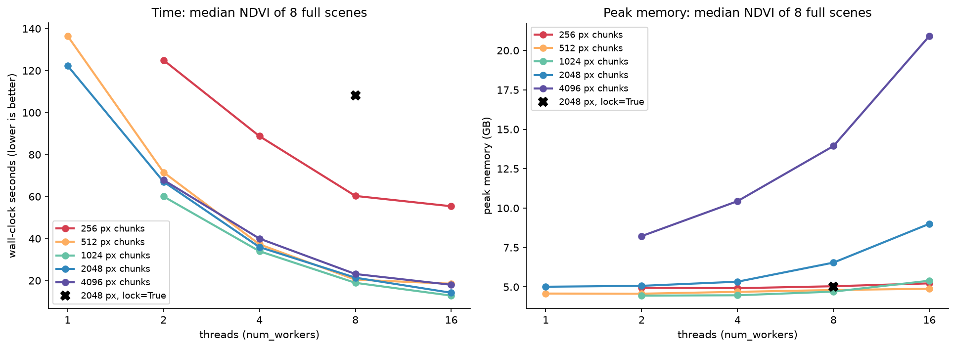

What the grid shows:

• Threads help almost linearly up to 8. With 2048 px chunks, 1 thread took 122 s and 8 threads 21 s, a speed-up of 5.7?; 16 threads took 14 s (8.6?). The gain flattens because the workstation has 16 physical cores, the reads compete for the disk cache, and other jobs were running.
• Tiny chunks are slow. 256 px chunks make a graph of 314,346 tasks, and the scheduler, not the CPU, becomes the bottleneck: 55 s on 16 threads, four times slower than 1024 px. If the task stream from Step 4 shows lots of thin bars and gaps, your chunks are too small.
• Big chunks are hungry. Peak memory is roughly a few 8-date blocks per thread. At 4096 px each block is 537 MB of float32 and its NDVI temporaries, so 16 threads needed 20.9 GB, more than eager NumPy needed for four dates. At 1024 px, memory stayed between 4.5 and 5.4 GB whatever the thread count.
• The sweet spot is broad. 512, 1024 and 2048 px chunks were within a few seconds of each other at each thread count. 1024 px on 16 threads was fastest (12.8 s); 2048 px on 8 threads (21 s, 6.5 GB) is a sensible default on an ordinary laptop.
• Check the read lock. By default (lock=None or True), rioxarray puts one shared lock around every read, so only one thread can read and decompress a block at a time, from any file. That is safe for any GDAL driver, but here it made the run five times slower (108 s against 21 s) and left the other seven threads waiting. Our open_stack passes lock=False, which opens a separate file handle for each read and is safe for local GeoTIFFs and COGs.
• A LocalCluster was no faster here. Four worker processes with two threads each took 21.2 s, the same as eight threads in one process. NumPy and GDAL release the GIL for the heavy work, so threads are enough. The distributed scheduler earns its start-up cost when tasks hold the GIL (pure-Python code), when you need its dashboard or memory limits, or when the work spreads over several machines.

The floor of about 4.5 GB, even on one thread, is mostly not dask. It includes the 482 MB result, Python and the libraries, and GDAL’s block cache, which by default may grow to 5% of physical memory (3.4 GB on this machine). Set the GDAL_CACHEMAX environment variable (for example to 512 MB) if you need a smaller footprint.

Step 7: write the result to disk chunk by chunk

For a result that is too big for memory, or one you simply want as a file, skip compute() and let rioxarray write it. With windowed=True, each chunk is written to its own window of the GeoTIFF as soon as it is computed. GDAL cannot write to one file from several threads at once, so pass a lock; the computation still runs in parallel, and only the writes take turns:

med = median_ndvi(*open_stack(DATES, 2048)).rio.write_nodata(np.nan, encoded=False)
with dask.config.set(scheduler="threads", num_workers=8):
    med.rio.to_raster(dest, tiled=True, blockxsize=512, blockysize=512, compress="deflate", predictor=3,
                      windowed=True, lock=threading.Lock())

wrote ndvi_median_2025_30UXC.tif: 370 MB on disk in 21.1 s; memory rose by at most 2.49 GB for a 482 MB result
check: 10980 x 10980 float32, EPSG:32630, deflate, 484 blocks of (512, 512)

The write took 21 seconds, about as long as computing the result in Step 4, and the process memory rose by at most 2.5 GB, against 6.6 GB when the result was gathered into memory. Each finished chunk goes to disk and is released, so this pattern works for results far larger than RAM. The file is a 370 MB deflate-compressed GeoTIFF with predictor=3 (the floating-point predictor), in 484 internal blocks of 512 px, the same block size as the inputs, so the next dask job can read it efficiently.

Two details are easy to miss. rio.write_nodata(np.nan, encoded=False) marks NaN as no data in the output, and out.attrs = {} in median_ndvi drops the input’s uint16 _FillValue, which would otherwise be written as a nodata value of 0 into a float file. To make the result a full Cloud Optimised GeoTIFF with overviews, write it with driver="COG" instead, which builds the overviews at the end, or add them afterwards with gdaladdo.

Pitfalls and limitations

• Chunks that split the file’s tiles. A chunk size that is not a multiple of the internal block size makes neighbouring chunks decompress the same blocks. Check src.block_shapes with rasterio, or gdalinfo, before choosing.
• Too many tasks. Every task costs the scheduler time. If len(arr.__dask_graph__()) runs into hundreds of thousands, use bigger chunks.
• Reductions across chunks. A median, percentile or sort along an axis needs that axis in one chunk; dask raises an error if it is not. Rechunk once, as in Step 3, rather than repeatedly.
• compute() loads the result. Dask keeps the inputs out of memory, not the output. If the result itself is too big, write it with to_raster, to_zarr or to_netcdf instead of computing it.
• Remote files. Reading COGs over HTTP from the Planetary Computer works with the same code, but each chunk then costs a network round trip, and the best chunk size and thread count change. The signed URLs also expire after about an hour, so long jobs need fresh ones.
• Memory numbers on Windows. We measured the resident set size of the process with psutil. The operating system and the memory allocator do not hand memory back immediately, so the memory curves show a high-water mark, not what dask is holding at each moment.
• Benchmarks are specific. These timings are for one workstation, one calculation and files on a local SSD. A different reduction, a network file system or a machine with less memory will give different best settings, so time your own pipeline on a sample before you run it on a large area.

Frequently asked questions

How do I process a large raster in Python without running out of memory?

Open it with rioxarray.open_rasterio(path, chunks=...) or xarray.open_dataset(..., chunks=...) so that it becomes a lazy dask array, write your calculation as normal, and either compute a result that fits in memory or write the result to disk with rio.to_raster(..., windowed=True, lock=...). Dask then streams the raster through memory in chunks. In this tutorial, eight full Sentinel-2 scenes went through in 6.4 GB, while eager NumPy needed 12.4 GB for four.

What chunk size should I use with dask and rioxarray?

Use a multiple of the file’s internal block size (512 px for Sentinel-2 COGs, often 256 or 512 for other GeoTIFFs), and aim for chunks of roughly 10–100 MB in the data type you compute in. For Sentinel-2 that means 1024 or 2048 px. In our tests 512, 1024 and 2048 px chunks were all within a few seconds of each other, 256 px chunks were four times slower, and 4096 px chunks needed up to 21 GB on 16 threads. Keep any axis you reduce over (such as time for a median) in a single chunk.

Is dask faster than NumPy for raster processing?

For data that fits in memory, NumPy on one core can be just as fast for simple element-wise maths, because NumPy has no scheduler overhead. Dask wins when the work is large enough to keep several threads busy, when reading and decompressing the files is a big part of the cost, or when the data does not fit in memory at all. Here dask was 5 to 6 times faster than eager NumPy, mostly because it read eight chunks in parallel.

Should I use the threaded scheduler or a dask distributed LocalCluster?

For one machine and raster maths built on NumPy and GDAL, start with the default threaded scheduler: those libraries release the GIL, so threads run in parallel, share memory and have no start-up cost. In our test a LocalCluster of 4 processes ? 2 threads took 21.2 s, the same as 8 threads. Use distributed when your tasks run pure-Python code that holds the GIL, when you want its live dashboard and per-worker memory limits, or when you scale out to a cluster. On Windows and macOS, create the cluster inside if __name__ == "__main__":, because worker processes are spawned by re-importing your script.

Can I use dask with rasterio directly, without xarray?

Yes, with dask.array.from_delayed or da.map_blocks and your own windowed reads, but you then manage coordinates, CRS and nodata yourself. rioxarray does that for you and keeps the georeferencing through every step, which is why it is the usual choice. For writing, rioxarray handles the windowed writes and the lock.

How do I see what dask is doing?

Wrap compute() in dask.diagnostics.ProgressBar() for a progress bar and Profiler() for a task stream, as in Step 4, or start a distributed.Client and open its dashboard (it needs Bokeh) to watch tasks, memory and workers live in the browser. arr.data.visualize() draws the task graph if Graphviz is installed.

Next steps

• Summarise the median NDVI by area: zonal statistics in Python works with chunked rasters too.
• Build a per-date series instead of one median: NDVI time series in Python with Sentinel-2 and odc-stac uses odc-stac, which returns the same kind of dask-backed DataArray.
• Run a neural network over a whole tile: deep learning inference on large rasters tiles a large image for a model, the same idea as chunks.
• Apply the same chunking to elevation: raster terrain analysis with rasterio computes slope and aspect, which need overlapping chunks (map_overlap in dask).
• Start with STAC and COGs: Sentinel-2 imagery of Lake Mead with STAC.
• Turn composites into an animation: satellite timelapse in Python builds one median composite per year.

Data and licences

• Sentinel-2 L2A: contains modified Copernicus Sentinel data 2025, processed by ESA. Bands B04 and B08 of tile 30UXC for eight dates, downloaded as Cloud Optimised GeoTIFFs from the Microsoft Planetary Computer on 3 November 2026. Copernicus Sentinel data are free and open under the Copernicus data licence.
• Code: dask_raster.py and raster_pipeline.py, tested with Python 3.12.0, dask 2026.8.0, distributed 2026.8.0, xarray 2026.9.0, rioxarray 0.23.0, rasterio 1.5.2, NumPy 2.5.4, pandas 3.1.0, matplotlib 3.11.2, networkx 3.7, psutil 7.2.2, pystac-client 0.9.1 and planetary-computer 1.0.0.