Mann-Kendall trend test on rasters in Python: Theil-Sen NDVI trends with xarray
Run a pixel-wise Mann-Kendall trend test and Theil-Sen slope on 24 years of MODIS NDVI in Python. Read MOD13A1 from the Microsoft Planetary Computer, mask it with the QA layer, aggregate to growing-season means, vectorise the tests with xarray.apply_ufunc (checked against pymannkendall), compare the seasonal and modified Mann-Kendall tests, control the false discovery rate across 229,229 pixels, and map greening and browning on China's Loess Plateau.
- Level
- Advanced
- Tested with
- Python 3.12
- Source code
- Download scripts
Key takeaways
- A pixel-wise trend analysis runs a Mann-Kendall test (is there a monotonic trend?) and a Theil-Sen slope (how steep is it?) on the time series at every pixel. Both are rank-based, so they cope with skewed data and outliers better than a least-squares fit.
- Aggregate before you test. Averaging 16-day MODIS NDVI to one May–September mean per year removes the seasonal cycle and most serial correlation: the median lag-1 autocorrelation falls from +0.57 for 16-day anomalies to +0.06 for annual means.
- Vectorised with NumPy and xarray.apply_ufunc, Mann-Kendall and Theil-Sen run on 229,229 pixels × 24 years in 2.2 s, and match pymannkendall exactly on sampled pixels.
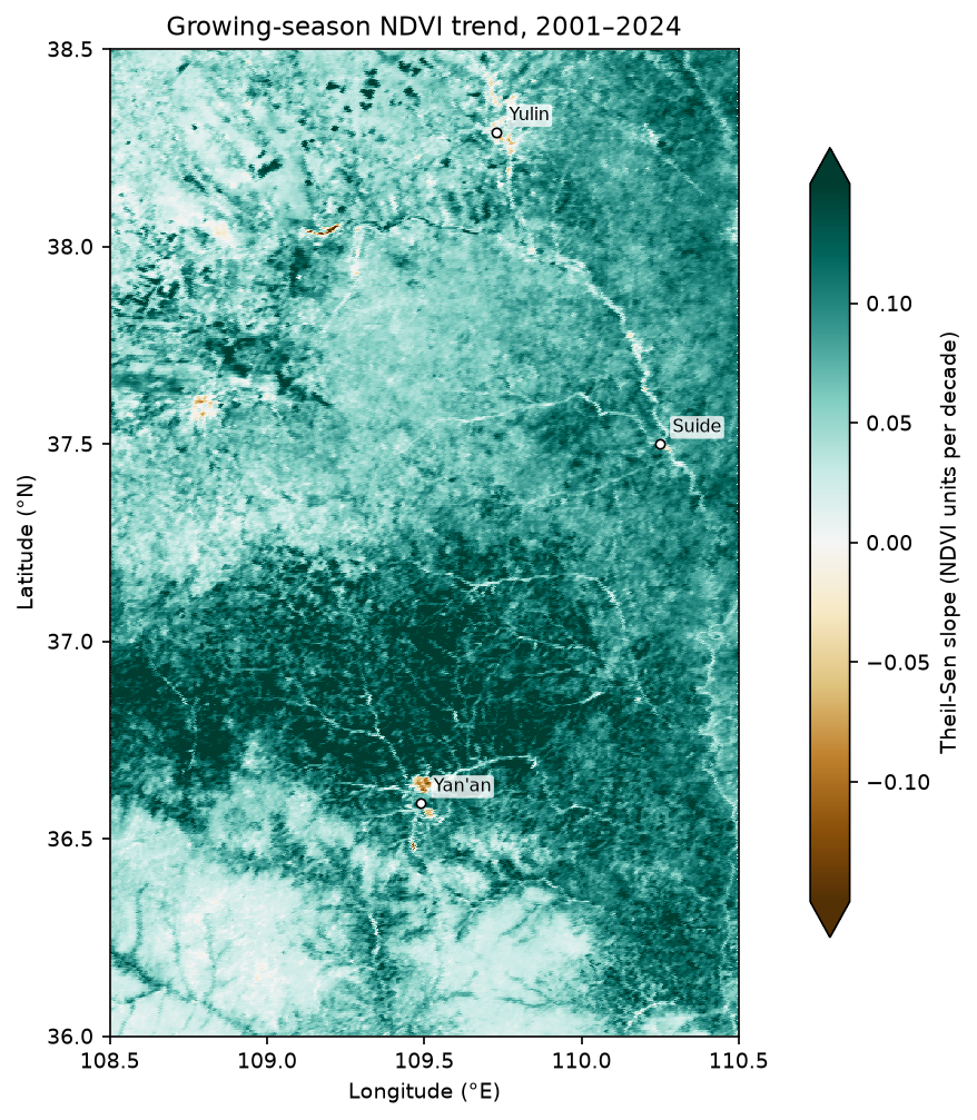
- Between Yan'an and Yulin on China's Loess Plateau, 97.7% of pixels show significant greening after Benjamini-Hochberg FDR control (q < 0.05), with a median slope of +0.080 NDVI per decade. Mean growing-season NDVI rose from 0.310 in 2001 to 0.517 in 2024. Only 261 pixels (0.1%) show significant browning.
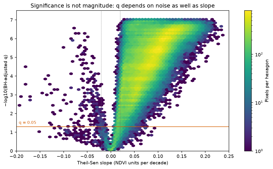
- Significance is not magnitude and a trend is not a mechanism. 3,848 pixels have a significant but tiny slope (under 0.02 per decade), and a pixel near Yan'an with an abrupt 2013 drop has a large slope but p = 0.21. Use breakpoint methods such as BFAST for abrupt change.
Before you start
- Comfortable with xarray DataArrays, groupby and resample (see the NDVI time series and ERA5 tutorials)
- Python 3.10+ with numpy, pandas, scipy, xarray, dask, rioxarray, rasterio, pystac-client, planetary-computer, pymannkendall, statsmodels and matplotlib
- An internet connection: the first run makes 1,140 windowed reads (about 1.5 GB of uncompressed pixels) from the Microsoft Planetary Computer, with no account needed
Short answer: to run a Mann-Kendall trend test on a raster time series in Python, load the stack as an xarray DataArray, mask bad-quality pixels, and aggregate to one value per year (for example the growing-season mean) to remove the seasonal cycle. Then write the test as a NumPy function over the last axis and apply it to every pixel with xarray.apply_ufunc. It returns the Mann-Kendall S, p-value and Theil-Sen slope per pixel; check it against pymannkendall on a few pixels. With one test per pixel, adjust the p-values with Benjamini-Hochberg FDR before you map significance. On 24 years of MODIS NDVI over China’s Loess Plateau, this flags 97.7% of 229,229 pixels as significantly greening, at a median +0.080 NDVI per decade.
“Is this area greening or browning, and where?” is one of the most common questions asked of satellite time series. The standard answer is a per-pixel Mann-Kendall test with a Theil-Sen slope. Both are simple, robust and easy to get subtly wrong: seasonality, serial correlation, cloud contamination, sensor changes and tens of thousands of simultaneous tests all affect the result. This tutorial does the whole analysis on real MODIS data, and every number below is printed by the script.
The study area is about 49,000 km² of northern Shaanxi, from Yan’an in the south to Yulin on the edge of the Mu Us sandy land. It is a good test case because it has one of the best-documented greening trends on Earth, linked to large-scale revegetation since China’s Grain for Green programme began in 1999, so you can judge whether the method finds what it should.
You will learn how to:
- search and read 24 years of MODIS MOD13A1 NDVI from the Microsoft Planetary Computer with
pystac-clientand windowedrasterioreads; - mask clouds and snow with the pixel reliability QA layer;
- reduce seasonality and autocorrelation by aggregating to growing-season means;
- write a vectorised Mann-Kendall and Theil-Sen function and run it with
xarray.apply_ufuncand dask; - cross-check against pymannkendall, and run the seasonal Mann-Kendall test;
- measure serial correlation and compare the modified MK and pre-whitening tests;
- apply Benjamini-Hochberg FDR correction across pixels and map significant greening and browning;
- see why significance is not magnitude, and where breakpoints break the method.
If you are new to satellite time series in xarray, the NDVI time series with ODC-STAC tutorial builds the basic cube. The ERA5 in Python with xarray tutorial covers the same groupby and resample patterns on climate data, and the trend code here works on ERA5-Land temperature without changes.
The data
MOD13A1 version 6.1 is the MODIS/Terra Vegetation Indices 16-Day L3 Global 500 m product. Each composite picks the best cloud-free observation of each pixel over 16 days, and stores NDVI (scaled by 10,000) with a pixel reliability layer. Terra has been collecting since February 2000, which gives one of the longest consistent NDVI records available at moderate resolution. The Microsoft Planetary Computer serves the whole archive as Cloud Optimised GeoTIFFs, with a STAC API and no account. Requests are signed with the planetary-computer package.
The full script is ndvi_trend_mann_kendall.py. It caches the data cube as a compressed .npz file in data/ after the first run, and writes figures to output/.
Step 1: read 25 years of MODIS composites
Search the modis-13A1-061 collection for the bounding box. Keep only Terra (MOD13A1) items, because Aqua’s MYD13A1 composites are offset by eight days and come from a different sensor. Read the same pixel window from every composite. Only the window is downloaded, not the full 2,400 × 2,400 tile, because the files are Cloud Optimised GeoTIFFs. A thread pool runs the requests in parallel.
BBOX = (108.5, 36.0, 110.5, 38.5)        # lon/lat: Yan'an (south) to Yulin (north), Shaanxi, ChinaYEARS = range(2001, 2025)                # 24 complete years (2025 is incomplete in the catalogue)SEASON = [5, 6, 7, 8, 9]                 # growing season, May-September
catalog = pystac_client.Client.open("https://planetarycomputer.microsoft.com/api/stac/v1",                                    modifier=planetary_computer.sign_inplace)items = catalog.search(collections=["modis-13A1-061"], bbox=BBOX,                       datetime=f"{YEARS[0]}-01-01/{YEARS[-1] + 1}-12-31").item_collection()items = sorted([it for it in items if it.id.startswith("MOD13A1")], key=lambda it: it.properties["start_datetime"])
with rasterio.open(items[0].assets["500m_16_days_NDVI"].href) as src:    crs = src.crs    win = from_bounds(*transform_bounds("EPSG:4326", crs, *BBOX, densify_pts=51), src.transform)    win = win.round_offsets().round_lengths()    transform = rasterio.windows.transform(win, src.transform)

def read(item):    out = []    for key in ("500m_16_days_NDVI", "500m_16_days_pixel_reliability"):        for attempt in range(5):            try:                with rasterio.open(item.assets[key].href) as src:                    out.append(src.read(1, window=win))                break            except rasterio.errors.RasterioIOError:                time.sleep(5 * (attempt + 1))                planetary_computer.sign_inplace(item)        else:            raise RuntimeError(f"could not read {item.id} {key}")    return out

with rasterio.Env(GDAL_DISABLE_READDIR_ON_OPEN="EMPTY_DIR", GDAL_HTTP_MAX_RETRY=5, GDAL_HTTP_RETRY_DELAY=2):    with ThreadPoolExecutor(16) as pool:        arrays = list(pool.map(read, items))
The script then stacks the arrays into an xarray.Dataset with time, y and x dimensions, drops duplicate dates, and lists any composites the catalogue lacks.
570 Terra composites, tiles ['h26v05'], 2000-12-18 .. 2025-12-19read 570 x 2 windows of 600 x 1076 pixels in 21 scube: 570 composites x 600 x 1076 pixels (500 m, MODIS sinusoidal); 7 duplicate composites (reprocessed copies) droppedcomposites missing from the catalogue: 2022-09-30, 2022-11-17, 2022-12-03, 2023-02-18, 2024-12-18, 2025-07-12, 2025-07-28, 2025-08-13, 2025-08-29, 2025-09-14, 2025-09-30, 2025-10-16, 2025-11-01-> 2025 lacks July-November, so the analysis uses 2001-2024 (24 growing seasons)Always check for gaps. The 2025 growing season is mostly missing from the catalogue, so including it would compare a full season with a partial one. A single missing composite in 2022 only removes one of about ten growing-season values for that year, which the averaging in Step 3 absorbs.
Step 2: mask clouds and snow with the QA layer
The pixel reliability layer gives a one-number quality summary per pixel and composite. Keep good (0) and marginal (1) values. Drop snow (2), cloud (3) and fill (−1), which would otherwise appear as spurious low NDVI. Then apply the 0.0001 scale factor, and date each composite by its mid-point rather than its start.
rel = cube.reliabilityfor k, name in [(-1, "fill / no data"), (0, "good"), (1, "marginal"), (2, "snow or ice"), (3, "cloudy")]: print(f" reliability {k:>2} ({name}): {float((rel == k).mean()):.1%} of pixel-composites in the window")ndvi = cube.ndvi.where((rel >= 0) & (rel <= 1) & (cube.ndvi > -2000)) * 1e-4ndvi = ndvi.assign_coords(time=cube.time + pd.Timedelta(days=8)) # date each composite by its mid-point reliability -1 (fill / no data): 0.0% of pixel-composites in the window reliability 0 (good): 80.3% of pixel-composites in the window reliability 1 (marginal): 15.6% of pixel-composites in the window reliability 2 (snow or ice): 1.1% of pixel-composites in the window reliability 3 (cloudy): 3.1% of pixel-composites in the windowThis is a semi-arid region, so only 4.2% of values are lost to snow and cloud. In a cloudier region, check that each pixel still has enough valid values per year after masking.
Step 3: aggregate to growing-season means
A 16-day NDVI series has a strong seasonal cycle, and consecutive composites are highly correlated. Both violate the Mann-Kendall test’s assumption of independent observations. The simplest fix is to aggregate: one May–September mean per year. Require at least 5 valid composites per season, drop pixels with a mean NDVI of 0.1 or less (water and bare sand), and keep only pixels with all 24 years.
The MODIS sinusoidal window is a parallelogram in longitude and latitude, so also mask out pixels whose centres fall outside the bounding box. The script also builds a monthly (year, month) array for the seasonal test in Step 5.
gs = ndvi.where(ndvi.time.dt.month.isin(SEASON), drop=True)n_valid = gs.notnull().groupby("time.year").sum()annual = gs.groupby("time.year").mean().where(n_valid >= 5) # need 5 of ~10 compositesmonthly = gs.resample(time="MS").mean()monthly = monthly.where(monthly.time.dt.month.isin(SEASON), drop=True)monthly = monthly.assign_coords(year=("time", monthly.time.dt.year.data), month=("time", monthly.time.dt.month.data))monthly = monthly.set_index(time=["year", "month"]).unstack("time").transpose("year", "month", "y", "x")mean_ndvi = annual.mean("year")years_ok = annual.notnull().sum("year")# the sinusoidal window is a parallelogram in lon/lat: keep only pixels whose centre is inside BBOXlon, lat = rasterio.warp.transform(crs, "EPSG:4326", *[a.ravel() for a in np.meshgrid(cube.x, cube.y)])lon = np.reshape(lon, mean_ndvi.shape); lat = np.reshape(lat, mean_ndvi.shape)inside = xr.DataArray((lon >= BBOX[0]) & (lon <= BBOX[2]) & (lat >= BBOX[1]) & (lat <= BBOX[3]), dims=("y", "x"))mean_ndvi = mean_ndvi.where(inside)land = inside & (mean_ndvi > 0.1) & (years_ok == len(YEARS))annual = annual.where(land)monthly = monthly.where(land)growing-season composites per year: 9.8 on average; median valid (QA-passed) per pixel-year inside the box 10pixels analysed: 229,229 of 229,233 inside the box (dropped: mean growing-season NDVI <= 0.1 or any year with < 5 valid composites)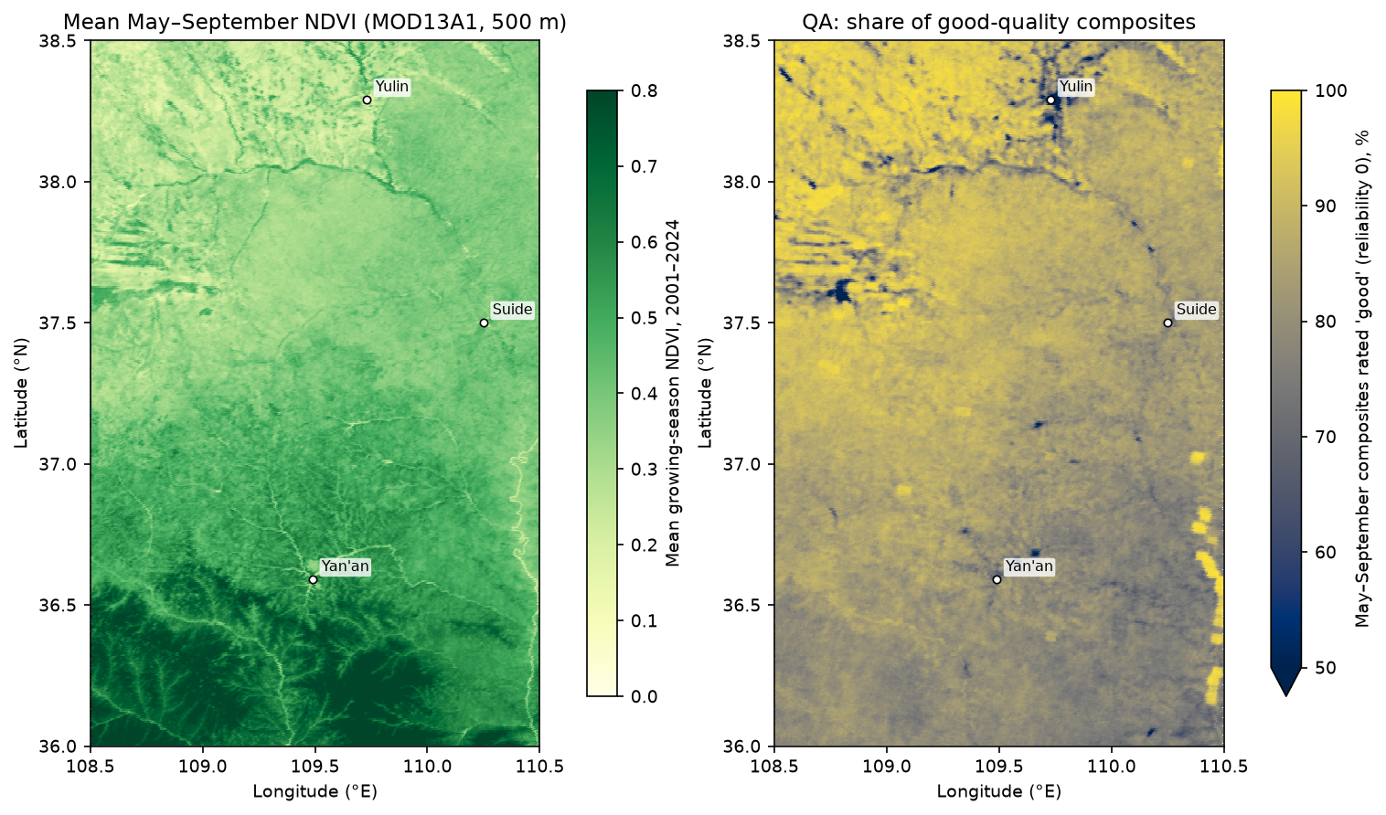
Step 4: vectorised Mann-Kendall and Theil-Sen with apply_ufunc
The Mann-Kendall statistic S is the sum of sign(xⱼ − xᵢ) over every pair of years in which year i comes before year j. Under the null hypothesis of no trend and independent values, S is approximately normal with mean 0 and variance n(n − 1)(2n + 5)/18. The Theil-Sen slope is the median of (xⱼ − xᵢ)/(tⱼ − tᵢ) over the same pairs. Both need all n(n − 1)/2 pairs, which is 276 pairs for 24 years. With np.triu_indices, you can compute all of them for every pixel at once, without a Python loop.
def mk_theil_sen(x, t):    """Mann-Kendall test and Theil-Sen slope along the last axis of x (time), for any leading shape.    Missing values are skipped pairwise. Variance ignores ties (fine for continuous NDVI means)."""    i, j = np.triu_indices(x.shape[-1], 1)    d = x[..., j] - x[..., i]    s = np.nansum(np.sign(d), axis=-1)    n = np.sum(~np.isnan(x), axis=-1)    var = n * (n - 1) * (2 * n + 5) / 18.0    z = np.where(s > 0, (s - 1) / np.sqrt(var), np.where(s < 0, (s + 1) / np.sqrt(var), 0.0))    p = 2 * norm.sf(np.abs(z))    slope = np.nanmedian(d / (t[j] - t[i]), axis=-1)    return np.stack([s, var, z, p, slope], axis=-1)

t_years = np.asarray(annual.year, dtype=float)stats = xr.apply_ufunc(mk_theil_sen, annual.chunk({"y": 64, "x": 64}), kwargs={"t": t_years},                       input_core_dims=[["year"]], output_core_dims=[["stat"]], dask="parallelized",                       output_dtypes=[float], dask_gufunc_kwargs={"output_sizes": {"stat": 5}})stats = stats.assign_coords(stat=["S", "varS", "z", "p", "slope"]).compute()p_mk = stats.sel(stat="p").where(land)slope = stats.sel(stat="slope").where(land) * 10                        # NDVI per decade
input_core_dims=[["year"]] tells xarray to move year to the last axis and pass each chunk to the function as a NumPy array of shape (y, x, year). output_core_dims=[["stat"]] adds a new five-element axis for the results. dask="parallelized" runs the 64 × 64-pixel chunks in parallel. The pairwise difference array for one chunk is 64 × 64 × 276 values, so memory stays small at any raster size.
Never trust a hand-written statistical test until you have compared it with a reference implementation. pymannkendall is slow per pixel, but it is the standard:
yy, xx = np.nonzero(land.values)pick = rng.choice(len(yy), 6, replace=False)for k in pick: series = annual.values[:, yy[k], xx[k]] ref = pmk.original_test(series) ours = stats.values[yy[k], xx[k]] print(f" ({yy[k]:>3},{xx[k]:>3}): S {ours[0]:+5.0f}/{ref.s:+5.0f} p {ours[3]:.4f}/{ref.p:.4f} " f"slope {ours[4]:+.5f}/{ref.slope:+.5f}")229,229 pixels in 2.2 scross-check with pymannkendall.original_test (pixel: S ours/pmk, p ours/pmk, slope ours/pmk): (394,830): S +158/ +158 p 0.0001/0.0001 slope +0.00771/+0.00771 (466,571): S +158/ +158 p 0.0001/0.0001 slope +0.00752/+0.00752 (262,408): S +184/ +184 p 0.0000/0.0000 slope +0.00669/+0.00669 (516,727): S +184/ +184 p 0.0000/0.0000 slope +0.00505/+0.00505 (265,611): S +180/ +180 p 0.0000/0.0000 slope +0.00901/+0.00901 ( 54,204): S +214/ +214 p 0.0000/0.0000 slope +0.00413/+0.00413The vectorised version processes all 229,229 pixels in 2.2 seconds and agrees with pymannkendall to every printed digit. Calling pmk.original_test in a loop over every pixel would take several minutes.
Step 5: the seasonal Mann-Kendall test
Annual means throw away within-season information. The seasonal Mann-Kendall test (Hirsch et al., 1982) keeps it without letting the seasonal cycle bias the result. It computes S separately for each season (here May, June, July, August and September), comparing each month only with the same month in other years, then sums the S values and their variances. The seasonal Sen slope is the median of all within-season pairwise slopes.
def seasonal_mk(x, t):    """Seasonal Mann-Kendall (Hirsch et al. 1982): x has dims (..., year, season). S and Var(S) are summed    over seasons; the slope is the median of all within-season pairwise slopes."""    i, j = np.triu_indices(x.shape[-2], 1)    s = var = 0    slopes = []    for m in range(x.shape[-1]):        xm = x[..., m]        d = xm[..., j] - xm[..., i]        s = s + np.nansum(np.sign(d), axis=-1)        n = np.sum(~np.isnan(xm), axis=-1)        var = var + n * (n - 1) * (2 * n + 5) / 18.0        slopes.append(d / (t[j] - t[i]))    z = np.where(s > 0, (s - 1) / np.sqrt(var), np.where(s < 0, (s + 1) / np.sqrt(var), 0.0))    p = 2 * norm.sf(np.abs(z))    slope = np.nanmedian(np.concatenate(slopes, axis=-1), axis=-1)    return np.stack([s, var, z, p, slope], axis=-1)

sstats = xr.apply_ufunc(seasonal_mk, monthly.chunk({"y": 64, "x": 64}), kwargs={"t": t_years}, input_core_dims=[["year", "month"]], output_core_dims=[["stat"]], dask="parallelized", output_dtypes=[float], dask_gufunc_kwargs={"output_sizes": {"stat": 5}})cross-check with pymannkendall.seasonal_test(period=5): (394,830): S +666/ +666 p 0.0000/0.0000 slope +0.00858/+0.00858 (466,571): S +699/ +699 p 0.0000/0.0000 slope +0.00724/+0.00724 (262,408): S +772/ +772 p 0.0000/0.0000 slope +0.00667/+0.00667annual MK and seasonal MK agree on the sign of the trend for 99.9% of pixels; p < 0.05 (unadjusted): annual 97.8%, seasonal 99.0%Here the two approaches agree on direction almost everywhere, and the seasonal test is slightly more powerful because it uses five values per year. The seasonal test earns its keep when a trend is confined to part of the year, such as earlier spring green-up, or when the series is monthly and you don’t want to collapse it. Note that it assumes the seasons are independent of one another. Consecutive months of NDVI are not, so treat its p-values as slightly optimistic.
Step 6: serial correlation, modified MK and pre-whitening
Positive serial correlation means each value carries less independent information than it appears to. The ordinary Mann-Kendall variance is then too small, so the test finds too many trends. First measure it: the lag-1 autocorrelation of the detrended series at every pixel.
def lag1(x):    """Lag-1 autocorrelation along the last axis after removing a least-squares linear trend."""    t = np.arange(x.shape[-1], dtype=float)    xd = x - np.nanmean(x, -1, keepdims=True)    tt = t - t.mean()    b = np.nansum(xd * tt, -1, keepdims=True) / np.sum(tt ** 2)    e = xd - b * tt    return np.nansum(e[..., 1:] * e[..., :-1], -1) / np.nansum(e ** 2, -1)

r1_annual = lag1(np.moveaxis(annual.values, 0, -1))[both]anom = ndvi.groupby("time.dayofyear") - ndvi.groupby("time.dayofyear").mean()   # 16-day deseasonalised anomaliesanom_v = np.moveaxis(anom.fillna(0).values, 0, -1)[both]r1_16day = lag1(anom_v)
tests = {"Original MK": pmk.original_test, "Hamed-Rao modified MK": pmk.hamed_rao_modification_test, "Yue-Wang modified MK": pmk.yue_wang_modification_test, "Pre-whitening (PW)": pmk.pre_whitening_modification_test, "Trend-free pre-whitening (TFPW)": pmk.trend_free_pre_whitening_modification_test}for name, f in tests.items(): ps = np.array([f(annual.values[:, yy[k], xx[k]]).p for k in sub])lag-1 autocorrelation, annual growing-season means: median +0.06; |r1| > 0.40 (approx. 5% test) for 13.7% of pixelslag-1 autocorrelation, 16-day deseasonalised anomalies: median +0.57 Original MK p < 0.05 for 97.6% of 2,000 random pixels Hamed-Rao modified MK p < 0.05 for 93.8% of 2,000 random pixels Yue-Wang modified MK p < 0.05 for 99.4% of 2,000 random pixels Pre-whitening (PW) p < 0.05 for 19.8% of 2,000 random pixels Trend-free pre-whitening (TFPW) p < 0.05 for 96.4% of 2,000 random pixels for contrast, MK on the 16-day anomaly series (547 values) of 500 pixels: p < 0.05 for 100.0% (original) vs 98.6% (Hamed-Rao)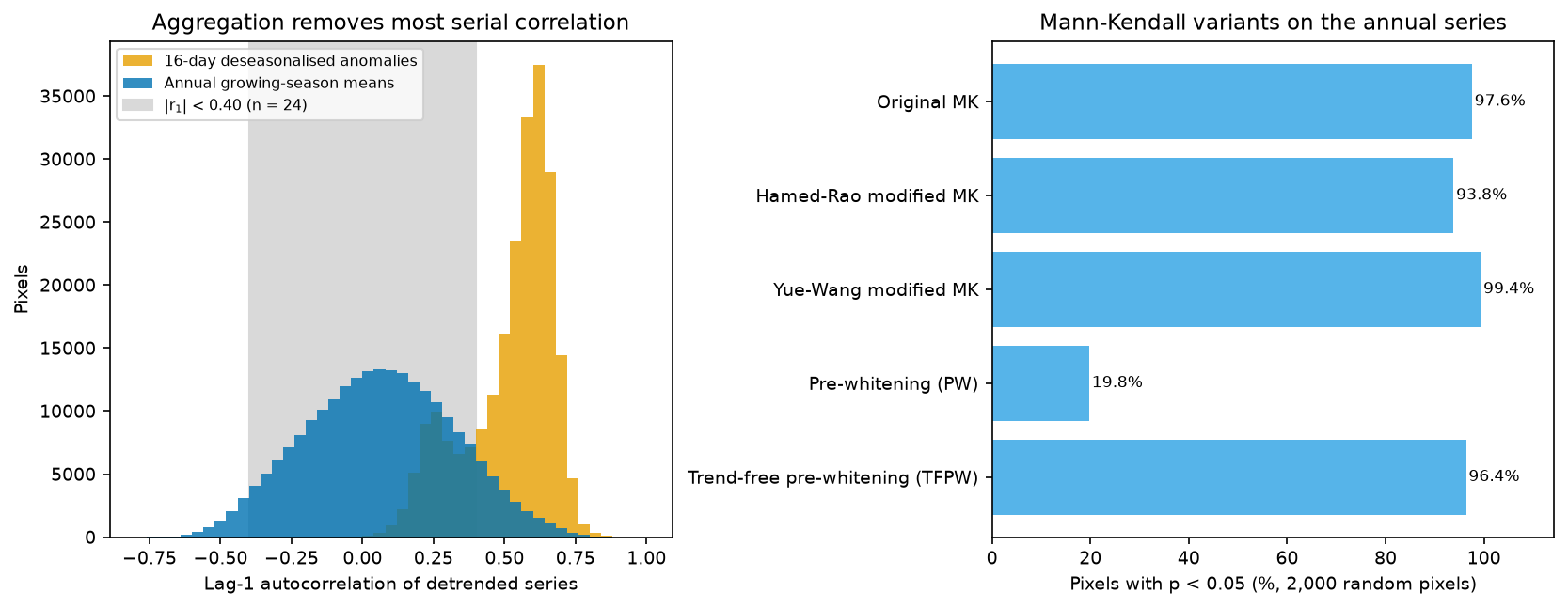
What this shows:
- Aggregation does most of the work. The 16-day anomalies have a median lag-1 autocorrelation of +0.57. The annual means have +0.06, and only 13.7% of pixels exceed the rough 5% significance threshold of ±0.40 (more than the 5% expected by chance, so some pixels do have multi-year swings worth a modified test).
- Variance-corrected tests change little here. The Hamed and Rao (1998) correction, which estimates an effective sample size from the significant autocorrelations of the ranks, lowers the significant share from 97.6% to 93.8%. The Yue and Wang (2004) correction raises it slightly, to 99.4%. Variance corrections can go either way, because negative autocorrelation makes the ordinary test conservative.
- Classic pre-whitening (PW) is the wrong tool for trended data. It fits the lag-1 autocorrelation to the raw series, so a strong trend looks like strong autocorrelation, and removing it also removes much of the trend: only 19.8% of pixels stay significant. Trend-free pre-whitening (Yue et al., 2002) removes the Sen slope first, whitens the residuals and then adds the trend back. It gives 96.4%.
A sensible default is to aggregate first, then report the original and a modified test (Hamed-Rao is a common choice) side by side. If they disagree materially, the autocorrelation matters and the modified test should be your primary result.
Step 7: control the false discovery rate across pixels
You have just run 229,229 hypothesis tests. At α = 0.05, even with no trend anywhere, you would expect about 11,461 false positives. The Benjamini-Hochberg procedure controls the false discovery rate, the expected proportion of false positives among the pixels you call significant. Sort the p-values, scale the k-th smallest by m/k, and take a running minimum from the top. The script implements it in five lines and checks it against statsmodels.
pv = p_mk.values[both]m = len(pv)order = np.argsort(pv)ranked = pv[order] * m / np.arange(1, m + 1)q = np.minimum.accumulate(ranked[::-1])[::-1]q_bh = np.empty(m); q_bh[order] = np.minimum(q, 1)q_sm = multipletests(pv, alpha=ALPHA, method="fdr_bh")[1]print(f"own Benjamini-Hochberg vs statsmodels: max |difference| in q = {np.abs(q_bh - q_sm).max():.2e}")own Benjamini-Hochberg vs statsmodels: max |difference| in q = 1.11e-16tests: 229,229; p < 0.05 unadjusted: 224,193 (97.8%); expected false positives if no trend anywhere: 11,461BH q < 0.05: 224,193 (97.8%); equivalent p-value threshold 0.0445Bonferroni p < 2.2e-07: 54,459 (23.8%)significant greening: 223,932 pixels (97.7%), median slope +0.080 NDVI/decadesignificant browning: 261 pixels (0.1%), median slope -0.038 NDVI/decadearea-mean Theil-Sen slope: +0.0803 NDVI/decade; mean growing-season NDVI 0.310 (2001) -> 0.517 (2024)significant but small (|slope| < 0.02/decade): 3,848; large (> 0.05/decade) but not significant: 123Benjamini-Hochberg changes nothing here, and that is a correct result, not a bug. BH adapts to how many real effects there are. When nearly every pixel has a strong trend, the BH threshold rises towards α itself (here, to p = 0.0445). There is also a quirk of small samples: with n = 24 the Mann-Kendall p-value can only take certain values. S = 82 gives p = 0.0445 and the next possible value, S = 80, gives p ≈ 0.050, so the BH cut-off falls between the same two values of S as the unadjusted 0.05. In a region with only a scattering of real trends, BH removes far more pixels.
Bonferroni, which controls the chance of even one false positive, keeps only 23.8% of pixels. That is far too strict for mapping, where a few false positives among 224,000 discoveries do no harm. The hot spot analysis tutorial covers the same trade-off for local spatial statistics.
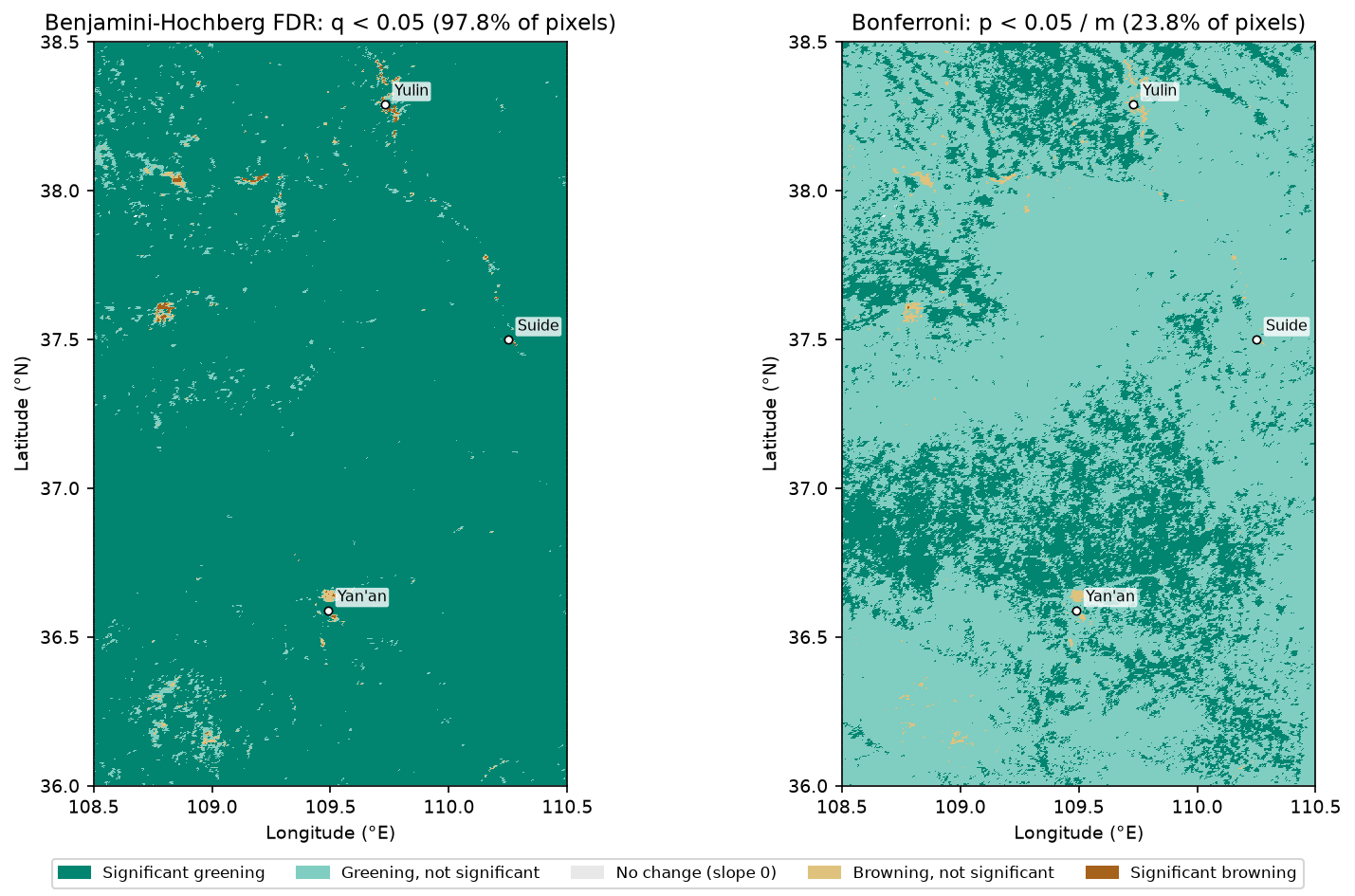
Over 24 years, mean growing-season NDVI rose from 0.310 to 0.517, and the area-mean Theil-Sen slope is +0.080 NDVI per decade. That matches the widely reported greening of the Loess Plateau. The test tells you there is a monotonic increase. It does not tell you why. Revegetation under Grain for Green, changes in rainfall, CO₂ fertilisation and farming practice all plausibly contribute, and separating them needs other data and other methods.
Step 8: look at the time series, and remember what the test cannot see
A map of p-values hides the shape of the change. Always plot some pixels. The script chooses four types: a strong significant greening, a significant browning, a large slope that is not significant, and a tiny slope that is significant.
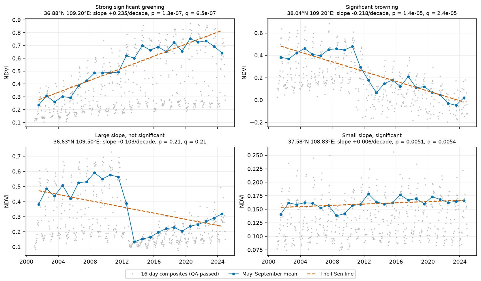
- Top left: a steady rise from about 0.24 to 0.75, the textbook case of a significant monotonic trend.
- Top right: stable NDVI until 2011, then a fall to about zero by the 2020s. A value near zero is typical of water or bare ground, so this is probably a surface change such as mining, construction or a new water body. Satellite imagery of the site would tell you which. The test calls it a significant browning trend, but the real story is a land-use change.
- Bottom left: near Yan’an, NDVI dropped from about 0.56 to 0.13 in a single year (2013), then recovered steadily. The timing and location are consistent with the large-scale levelling of loess hills for Yan’an’s new urban district, but check that against imagery before you rely on it. Mann-Kendall sees a fall followed by a rise, so S is small and p = 0.21, even though the slope is −0.103 per decade. Neither number describes what happened. This is a breakpoint. Use methods built for that, such as BFAST (Verbesselt et al., 2010), which splits a series into segments with separate trends and seasonal terms, or tools such as LandTrendr and CCDC.
- Bottom right: a sandy pixel near the Mu Us edge, where NDVI rose from about 0.15 to 0.17. It is significant (p = 0.0051) because the series is smooth, but a change of 0.006 per decade is ecologically negligible and within plausible sensor drift.
That last point is general. A p-value depends on the slope and the noise. A clean small trend can be highly significant, and a large noisy one not significant at all.
Step 9: check sensitivity to the end of the series
Terra’s orbit has been drifting since 2020, as the satellite nears the end of its mission, so its overpass time is getting earlier. That can shift NDVI slightly through changes in illumination and view geometry. A simple robustness check is to re-run the test on 2001–2019 only:
st19 = mk_theil_sen(np.moveaxis(annual.sel(year=slice(2001, 2019)).values, 0, -1)[both], t_years[:19])sig19 = st19[:, 3] < ALPHA2001-2019: p < 0.05 for 96.8% of pixels (full series 97.8%); slope correlation with 2001-2024 0.93; same sign 99.7%The pattern is essentially unchanged: 96.8% of pixels are significant, the slopes correlate at 0.93, and 99.7% keep the same sign. The recent years are not driving the result.
Limitations and honest caveats
- Monotonic is an assumption. Mann-Kendall tests for a consistent increase or decrease. It has little power against U-shapes, steps or recoveries, and Theil-Sen forces a straight line through them. Plot the series, and use breakpoint methods such as BFAST for abrupt change.
- Significance ≠ magnitude ≠ importance. Report the slope with its units next to the p-value or q-value, and decide in advance what size of change matters for your question.
- Sensor effects. MODIS Collection 6.1 corrected the worst of Terra’s earlier calibration drift, but orbit drift since 2020 and the change from the 2000s to newer sensors still matter for small trends. Collection changes, gaps (2022 and 2025 here) and compositing artefacts can all mimic trends. Cross-check against an independent record, such as Aqua MODIS, VIIRS or Landsat, when small trends matter.
- QA masking is a choice. Keeping marginal values (reliability 1) adds data but some noise. Dropping them in a cloudy region can leave too few observations, or bias the seasonal mean towards clear-sky days.
- Spatial autocorrelation. Neighbouring pixels are not independent tests. Benjamini-Hochberg remains valid under positive dependence, but the 229,229 tests contain far less independent information than their number suggests. Treat clusters, not single pixels, as the unit of interpretation.
- NDVI saturates over dense vegetation, so trends in the forested south are under-stated relative to the sparser north.
- Correlation is not causation. The greening matches the timing of the Grain for Green programme, but this analysis alone cannot attribute it.
Frequently asked questions
How do I run a Mann-Kendall test on every pixel of a raster in Python?
Load the raster stack as an xarray DataArray with a time dimension, write the test as a NumPy function that works along the last axis (as mk_theil_sen above does), and call xarray.apply_ufunc(func, da, input_core_dims=[["time"]], output_core_dims=[["stat"]], dask="parallelized"). Looping pymannkendall.original_test over every pixel also works, but it is much slower. Use it to check your vectorised version on a few pixels.
What is the difference between Mann-Kendall and Sen’s slope?
Mann-Kendall is a hypothesis test: it tells you whether there is evidence of a monotonic trend, with a p-value. Sen’s slope (the Theil-Sen estimator) measures how fast the value changes, in data units per unit time, as the median of all pairwise slopes. You normally report both: the slope for magnitude and the test for confidence.
Should I use the seasonal Mann-Kendall test or aggregate to annual values?
If you only care about the overall trend, aggregating to one value per year (an annual or growing-season mean) is simpler. It also removes most serial correlation. Use the seasonal Mann-Kendall test when you have sub-annual data and the trend might differ between seasons, or when you want to keep the extra observations. Both should give the same direction when the trend is strong, as they did for 99.9% of pixels here.
How do I deal with autocorrelation in a Mann-Kendall trend test?
First reduce it by aggregating to annual values. Then measure the lag-1 autocorrelation of the detrended series. If it is material, use a variance-corrected test such as the Hamed-Rao or Yue-Wang modified Mann-Kendall, or trend-free pre-whitening. Avoid classic pre-whitening on strongly trended series, because it removes part of the trend: here it cut the significant share from 97.6% to 19.8%.
Do I need a multiple-testing correction for a pixel-wise trend analysis?
Yes, if you map significance. With hundreds of thousands of pixels, a 5% threshold produces thousands of false positives even where nothing changes. The Benjamini-Hochberg false discovery rate correction is the usual choice. Bonferroni is too strict for maps. Report how many pixels pass before and after correction.
Is MODIS NDVI good enough for long-term trend analysis?
For regional trends of a few hundredths of NDVI per decade, yes: MOD13A1 v6.1 has a consistent processing chain from 2000 to the present. For very small trends, check the sensitivity to Terra’s post-2020 orbit drift (as in Step 9), cross-check with Aqua, VIIRS or Landsat, and mask with the QA layer. For field-scale change, use Landsat or Sentinel-2.
Next steps
- Build a cleaner NDVI cube from Sentinel-2 or Landsat in the NDVI time series with ODC-STAC tutorial, and run
mk_theil_senon its annual means. - Swap NDVI for ERA5-Land air temperature or precipitation from the ERA5 in Python with xarray tutorial. The trend code works unchanged on any
(time, y, x)cube. - If you classify the trends into land cover change, assess the result with the stratified estimators in the land cover accuracy assessment tutorial.
- To test whether significant pixels cluster in space, see hot spot analysis with Getis-Ord Gi*.
Data and licences
- MODIS MOD13A1 v061: Didan, K. (2021). MODIS/Terra Vegetation Indices 16-Day L3 Global 500m SIN Grid V061. NASA EOSDIS Land Processes Distributed Active Archive Center. NASA LP DAAC data are freely available without restriction. Accessed via the Microsoft Planetary Computer.
References: Mann, H. B. (1945) Econometrica, 13, 245–259. Kendall, M. G. (1975) Rank Correlation Methods, 4th edn. Griffin. Sen, P. K. (1968) Journal of the American Statistical Association, 63, 1379–1389. Hirsch, R. M., Slack, J. R. and Smith, R. A. (1982) Water Resources Research, 18, 107–121. Hamed, K. H. and Rao, A. R. (1998) Journal of Hydrology, 204, 182–196. Yue, S. and Wang, C. Y. (2004) Water Resources Management, 18, 201–218. Yue, S., Pilon, P., Phinney, B. and Cavadias, G. (2002) Hydrological Processes, 16, 1807–1829. Benjamini, Y. and Hochberg, Y. (1995) Journal of the Royal Statistical Society B, 57, 289–300. Verbesselt, J., Hyndman, R., Newnham, G. and Culvenor, D. (2010) Remote Sensing of Environment, 114, 106–115.
The full script is ndvi_trend_mann_kendall.py. It was tested on Python 3.12.0 with numpy 2.5.4, pandas 3.1.0, scipy 1.18.1, xarray 2026.9.0, dask 2026.8.0, rasterio 1.5.2, pystac-client 0.9.1, planetary-computer 1.0.0, pymannkendall 1.4.3 and statsmodels 0.15.0 on 27 October 2026.
Key terms
- Mann-Kendall test
- A non-parametric test for a monotonic trend. It counts how many later values are higher than earlier ones minus how many are lower (the statistic S) and compares S with its distribution under no trend.
- Theil-Sen slope (Sen's slope)
- The median of the slopes between every pair of points in a time series. It is a robust estimate of the rate of change, in data units per unit time.
- Seasonal Mann-Kendall
- The Hirsch et al. (1982) extension that computes S separately for each season (for example each month) and sums them, so a seasonal cycle is never compared with itself across seasons.
- Serial correlation
- Correlation between successive values in a time series. Positive serial correlation makes the ordinary Mann-Kendall test find too many significant trends.
- Modified Mann-Kendall test
- A version of the test that inflates or deflates the variance of S to account for serial correlation, such as Hamed and Rao (1998) or Yue and Wang (2004).
- Pre-whitening
- Removing lag-1 autocorrelation from a series before testing. Trend-free pre-whitening (TFPW) removes the trend first, so the whitening does not also remove part of the trend.
- False discovery rate (FDR)
- The expected share of false positives among results called significant. The Benjamini-Hochberg procedure controls it across many tests, such as one test per pixel.
- Pixel reliability
- The MODIS vegetation index quality summary layer: 0 good, 1 marginal, 2 snow or ice, 3 cloudy, -1 fill.
Data for this tutorial
- Microsoft Planetary Computer · Hosts the MODIS MOD13A1 v6.1 16-day 500 m vegetation indices collection used here, with a free STAC API
- NASA Earthdata · The original LP DAAC distribution of MOD13A1 and its user guide
Licences and formats for each source are listed in the GIS data sources catalogue.