Land cover accuracy assessment in Python: confusion matrix, Olofsson area estimates and sample size
Assess a real land cover map in Python: ESA WorldCover 2021 against 8,597 Eurostat LUCAS 2022 field survey points in Ireland. Build the confusion matrix, compute overall, user's and producer's accuracy, see why kappa is discouraged, and use the Olofsson et al. (2014) stratified estimators to get error-adjusted areas with 95% confidence intervals and to plan a new stratified random sample.
- Level
- Advanced
- Tested with
- Python 3.12
- Source code
- Download scripts
Key takeaways
- An accuracy assessment compares a map with better reference data at sample locations. The confusion matrix gives overall accuracy, user's accuracy (how reliable each map class is) and producer's accuracy (how much of each real class the map captures).
- Against 8,597 LUCAS 2022 field survey points, ESA WorldCover 2021 has an area-weighted overall accuracy of 0.664 ± 0.012 in Ireland. Counting agreeing points naively gives 0.705, because LUCAS over-samples arable land and under-samples grassland.
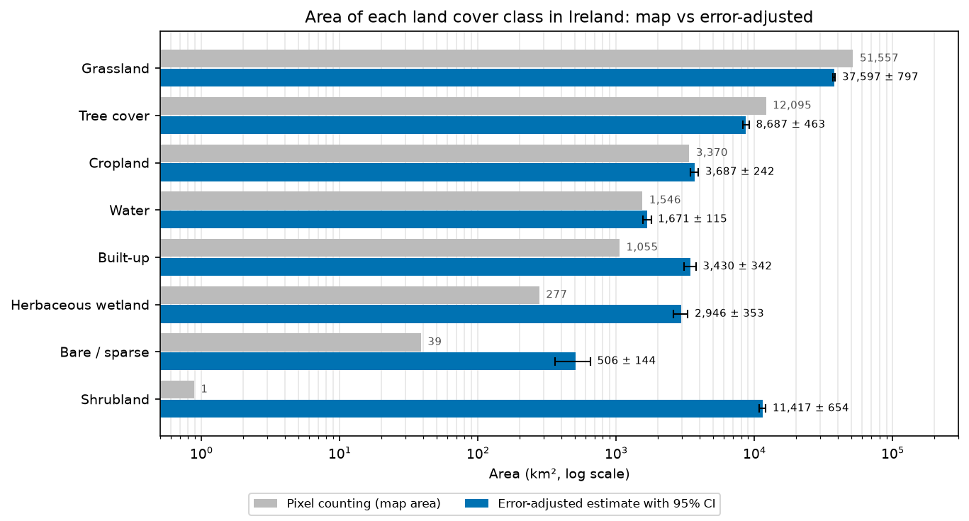
- Pixel counting is a biased area estimator. The map says Ireland is 73.7% grassland (51,557 km²); the error-adjusted estimate is 37,597 ± 797 km². Heath, bog and scrub that WorldCover labels as grassland add up to an estimated 11,417 ± 654 km² of shrubland and 2,946 ± 353 km² of herbaceous wetland.
- Use the stratified estimators of Olofsson et al. (2014): weight each row of the error matrix by the mapped area of its class. Report user's and producer's accuracy and areas with confidence intervals, and skip kappa (Pontius and Millones, 2011).
- For a new design, Cochran's formula gives n = 2,171 points for a standard error of 0.01 on overall accuracy. A compromise allocation with at least 100 points per class keeps that standard error at 0.0113 while making every class's user's accuracy estimable.
Before you start
- Comfortable with NumPy, pandas and reading rasters with rasterio (see the land cover classification tutorial)
- Python 3.10+ with numpy, pandas, geopandas, rasterio, shapely, pyproj, matplotlib, openpyxl and requests
- About 2 GB of free disk space: the script downloads five WorldCover tiles (about 1.4 GB), the LUCAS 2022 survey for Ireland and the LUCAS master grid on the first run
Short answer: to assess the accuracy of a land cover map in Python, read the map class at each reference point, cross-tabulate map against reference in a confusion matrix, and then turn the counts into area proportions by weighting each map class (row) by its share of the mapped area. That gives the unbiased overall, user’s and producer’s accuracy and error-adjusted class areas with 95% confidence intervals of Olofsson et al. (2014). Don’t report kappa. For ESA WorldCover 2021 in Ireland, checked against 8,597 Eurostat LUCAS 2022 survey points, overall accuracy is 0.664 ± 0.012, and the true grassland area is about 37,600 km², not the 51,557 km² you get by counting pixels.
A land cover map without an accuracy assessment is a picture, not a measurement. Every map has errors, and those errors are not random: they pile up in particular classes, and they bias any area you read off the map. The good news is that the statistics for doing this properly are settled, short and easy to code. This tutorial assesses a real global product against real independent field data, with every number below printed by the script.
The reference data are not a textbook sample, which makes this a useful worked example. LUCAS was not designed to validate WorldCover, so you will see how to post-stratify it, why its unequal selection rates need design weights, and how the point-vs-pixel and date mismatches affect the result.
You will learn how to:
- compute class areas by pixel counting on a 10 m map in geographic coordinates;
- build a legend crosswalk from the LUCAS land cover nomenclature to the WorldCover classes;
- derive design weights for LUCAS from the master grid, and post-stratify it by map class;
- read the confusion matrix, and compute overall, user’s and producer’s accuracy;
- see why kappa is discouraged, and use quantity and allocation disagreement instead;
- produce an area-adjusted error matrix and error-adjusted areas with 95% confidence intervals;
- check the point-vs-pixel, observation-type and date caveats;
- plan the sample size and allocation for a new stratified random sample, and draw it.
If you need a map to assess, the random forest land cover classification tutorial and the habitat mapping series both produce one. Everything here applies to your own maps unchanged.
The data
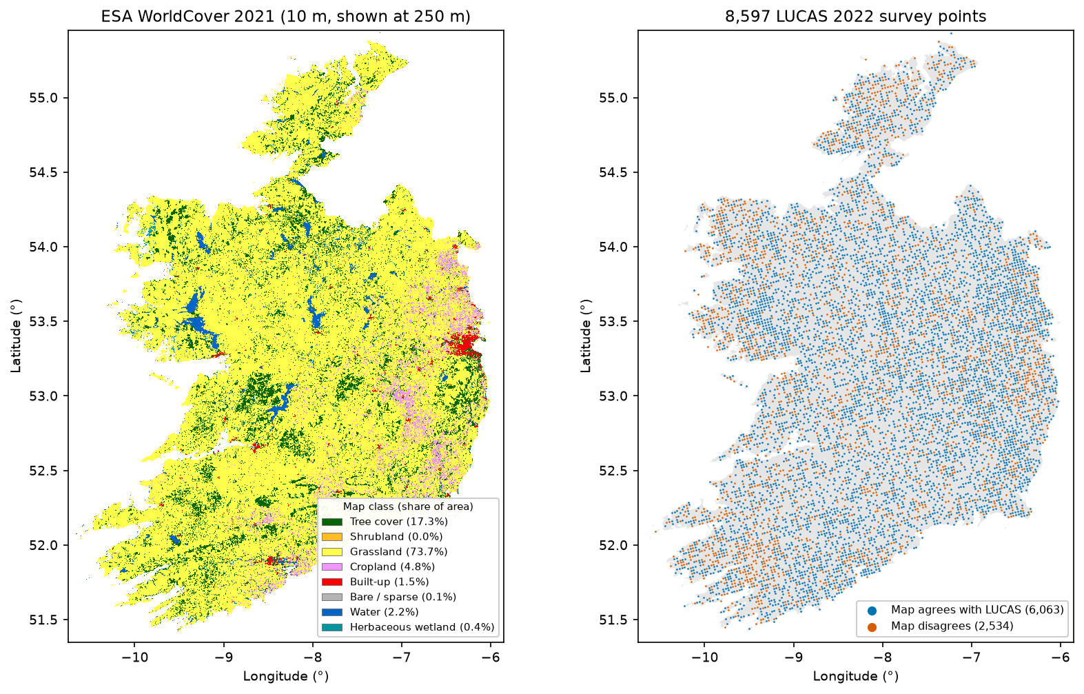
- ESA WorldCover 2021 v200: a global 10 m land cover map with 11 classes, made from Sentinel-1 and Sentinel-2 data from 2021. It is distributed as 3° × 3° Cloud Optimised GeoTIFF tiles in EPSG:4326 on AWS, with no login. Ireland needs five tiles.
- Eurostat LUCAS 2022: the Land Use/Cover Area frame Survey. Surveyors visit (or photo-interpret) points on a 2 km grid across the EU and record the land cover at the point, using a detailed three-level legend. Ireland has 8,597 points in the 2022 survey. Eurostat publishes the microdata per country as CSV.
- The LUCAS master grid: the full 2 km grid, including which points were selected for 2022 and the 2018 photo-interpretation stratum of every point. You need it to work out the selection probabilities.
- GISCO NUTS 2021 boundaries for the outline of Ireland.
The full script is accuracy_assessment.py. It caches all downloads in data/ and writes its figures and tables to output/.
Step 1: the map and the study area
Download the NUTS 0 polygon for Ireland and work out which WorldCover tiles it touches. Tiles are named by their south-west corner on a 3° grid.
WC_URL = "https://esa-worldcover.s3.eu-central-1.amazonaws.com/v200/2021/map/ESA_WorldCover_10m_2021_v200_{}_Map.tif"NUTS_URL = "https://gisco-services.ec.europa.eu/distribution/v2/nuts/geojson/NUTS_RG_01M_2021_4326_LEVL_0.geojson"
nuts = gpd.read_file(download(NUTS_URL, DATA / "NUTS_RG_01M_2021_4326_LEVL_0.geojson"))ireland = nuts[nuts.NUTS_ID == "IE"].to_crs("EPSG:4326")ie_geom = ireland.geometry.iloc[0]x0, y0, x1, y1 = ie_geom.boundstiles = [f"N{lat:02d}W{-lon:03d}" for lat in range(int(np.floor(y0 / 3) * 3), int(y1) + 1, 3) for lon in range(int(np.floor(x0 / 3) * 3), int(x1) + 1, 3)]tiles = [t for t in tiles if box(-int(t[4:]), int(t[1:3]), -int(t[4:]) + 3, int(t[1:3]) + 3).intersects(ie_geom)]paths = {t: download(WC_URL.format(t), DATA / f"WorldCover_2021_{t}.tif") for t in tiles}Ireland (NUTS IE, 1:1M): bounds -10.66..-6.00 E, 51.42..55.44 N, geodesic area 69,940 km2WorldCover 2021 v200 tiles: N51W012, N51W009, N51W006, N54W012, N54W009Step 2: class areas by pixel counting
The stratified estimators need the mapped area of each class, so count pixels first. WorldCover is in degrees, and a 10 m pixel (1/12,000°) gets narrower towards the pole: at 55° N it covers about 8% less ground than at 51.5° N. So compute the ellipsoidal area of one pixel in each row and multiply the class counts row by row. The script reads 3,000-row windows, masks them to the polygon, and uses one np.bincount per window to count classes per row.
def row_areas(transform, row0, nrows):    """Ellipsoidal area (m2) of one pixel in each row: 10 m pixels in EPSG:4326 shrink towards the pole."""    lat_top = transform.f + transform.e * np.arange(row0, row0 + nrows)    lat_bot = lat_top + transform.e    lon0, lon1 = 0.0, transform.a    return np.array([abs(geod.polygon_area_perimeter([lon0, lon1, lon1, lon0], [t, t, b, b])[0])                     for t, b in zip(lat_top, lat_bot)])

STEP = 3000 # rows per window: 3000 x 36000 pixelsarea_m2 = np.zeros(256)pix = np.zeros(256, dtype=np.int64)win_counts = [] # per-window class counts, for sampling in Step 8for t, p in paths.items(): with rasterio.open(p) as src: for r0 in range(0, src.height, STEP): win = Window(0, r0, src.width, min(STEP, src.height - r0)) wb = rasterio.windows.bounds(win, src.transform) part = ie_geom.intersection(box(*wb)) if part.is_empty: continue wt = rasterio.windows.transform(win, src.transform) inside = geometry_mask([part], out_shape=(win.height, win.width), transform=wt, invert=True) arr = src.read(1, window=win) rows = np.nonzero(inside)[0] cls = arr[inside] counts = np.bincount(rows * 256 + cls, minlength=win.height * 256).reshape(win.height, 256) area_m2 += (counts * row_areas(src.transform, r0, win.height)[:, None]).sum(0) pix += counts.sum(0) win_counts.append((t, r0, win.height, counts.sum(0)))1,353,687,446 pixels inside Ireland; mapped area 69,940 km2 (nodata pixels: 0) class pixels area_km2 W10 Tree cover 233,874,437 12,095.3 0.172920 Shrubland 16,894 0.9 0.000030 Grassland 998,316,939 51,557.0 0.737240 Cropland 64,800,106 3,370.2 0.048250 Built-up 20,380,643 1,054.7 0.015160 Bare / sparse 750,160 38.6 0.000680 Water 30,125,439 1,546.1 0.022190 Herbaceous wetland 5,422,828 277.4 0.0040Moss and lichen covers only 199 pixels, so the script merges it into bare / sparse. The column W is the stratum weight: the share of the mapped area in each class. Note how lopsided it is. WorldCover calls almost three-quarters of Ireland grassland and maps less than 1 km² of shrubland.
Step 3: the LUCAS reference data and the legend crosswalk
LUCAS records land cover with a three-level code (SURVEY_LC1): A artificial, B cropland, C woodland, D shrubland, E grassland, F bare land, G water and H wetlands, each with sub-classes. WorldCover has eleven broad classes. The crosswalk is the most consequential choice you will make, so write it as an explicit function and print it.
def lucas_to_worldcover(lc1, lu1):    """Crosswalk from the LUCAS 2022 land cover legend (LC1) to the ESA WorldCover legend."""    a, two = lc1[0], lc1[:2]    if a == "A":        return 50                                 # roofed and non-roofed artificial surfaces    if a == "B":        if lc1 == "B55":            return 30                             # temporary grassland (sown ley): WorldCover sees grass        if two == "B7":            return 10                             # fruit trees        if two == "B8" or lc1 == "Bx2":            return 20                             # vineyards, nurseries and other permanent woody crops        return 40                                 # arable crops, incl. Bx1 (arable land, photo-interpreted)    if a == "C":        return 10                                 # broadleaved, coniferous and mixed woodland    if a == "D":        return 20    if a == "E":        return 30    if a == "F":        if lc1 == "F40" and str(lu1).startswith("U11"):            return 40                             # bare arable soil between crops (agricultural use)        return 60                                 # rocks, sand, lichens and moss (F30), other bare soil    if a == "G":        return 70 if lc1 == "G50" else 80    if a == "H":        return 60 if lc1 in ("H22", "H23") else 90   # salines and intertidal flats are unvegetated    raise ValueError(lc1)

lucas = pd.read_csv(download(LUCAS_URL, DATA / "IE_LUCAS_2022.csv"), low_memory=False)lucas["ref"] = [lucas_to_worldcover(a, b) for a, b in zip(lucas.SURVEY_LC1, lucas.SURVEY_LU1)]8,597 LUCAS 2022 points in Ireland, surveyed 09 May 2022 .. 09 Feb 2023 observation type 1 (field, <= 100 m): 3,933 observation type 2 (field, > 100 m): 205 observation type 3 (photo-interpreted in the field): 161 observation type 7 (photo-interpreted in the office): 4,298crosswalk LUCAS LC1 -> WorldCover: Tree cover <- B71 C C10 C20 C21 C22 C23 C30 C31 C32 C33 Shrubland <- B83 B84 D10 D20 Grassland <- B55 E10 E20 E30 Cropland <- B11 B12 B13 B14 B15 B16 B21 B22 B23 B32 B37 B41 B43 B51 B52 B53 B54 Bx1 F40 Built-up <- A11 A12 A13 A21 A22 A30 Bare / sparse <- F10 F20 H23 Water <- G11 G21 G30 G40 Herbaceous wetland <- H11 H12 H21F40 bare soil on agricultural land counted as cropland: 74; B55 temporary grassland counted as grassland: 76Three of these decisions deserve a sentence each:
- Temporary grassland (B55) is sown grass in an arable rotation. LUCAS files it under cropland because of how the land is managed, but from space it looks exactly like grass. WorldCover’s cropland definition is about cultivated annual crops, so B55 goes to grassland.
- Bare arable soil (F40 with agricultural land use) is a ploughed field between crops. It goes to cropland, because that is what WorldCover is trying to map there.
- Peat bog (H12) and inland marsh (H11) go to herbaceous wetland. Heathland (D10, D20) goes to shrubland. In Ireland, much heath sits on blanket peat, and LUCAS and WorldCover draw the heath/bog/grass boundaries differently. Keep that in mind when you read the shrubland and wetland results.
Step 4: LUCAS is not a map-stratified sample, so weight it
The Olofsson estimators assume a probability sample in which you know each point’s chance of selection. LUCAS 2022 is a probability sample, but not one stratified by WorldCover. Eurostat selects points from the 2 km master grid at different rates in different strata, which come from a 2018 photo-interpretation of every grid point. The master grid records both the stratum (STR18) and whether each point was selected for 2022 (LUCAS_FLAG), so you can rebuild the selection rates.
grid = pd.read_csv(grid_csv)grid = grid[grid.NUTS0_21 == "IE"]grid["cell"] = grid.NUTS2_21 + "_S" + grid.STR18.astype(str)cells = grid.groupby("cell").agg(N=("POINT_ID", "size"), n=("LUCAS_FLAG", "sum"))cells["w"] = cells.N / cells.n.replace(0, np.nan)lucas = lucas.merge(grid[["POINT_ID", "cell", "STR18", "LUCAS_FLAG"]], on="POINT_ID", how="left")lucas["w"] = lucas.cell.map(cells.w)master grid: 17,458 points on the 2 km grid in Ireland, 8,597 in the 2022 sampleselection rate by 2018 photo-interpretation stratum (STR18): 1 arable 3,649 of 4,146 (88%) 2 permanent crops 11 of 11 (100%) 3 grass 1,903 of 6,898 (28%) 4 wooded 1,094 of 2,753 (40%) 5 shrubs 830 of 2,083 (40%) 6 bare/rare vegetation 365 of 504 (72%) 7 artificial 341 of 600 (57%) 8 inland water 335 of 368 (91%) 9 transitional/coastal water 0 of 23 (0%) 10 impossible to PI 69 of 72 (96%)design cells (NUTS 2 x STR18): 30; weights 1.00 .. 6.03; sum of weights 17,435 = grid points represented (x 4 km2 = 69,740 km2)grid points in cells with no sample (not represented): 23Arable points were selected at 88%, grass points at only 28%. Unweighted, LUCAS over-represents arable land about three-fold relative to grassland. Each point’s design weight is the inverse of its selection rate within its cell (NUTS 2 region × stratum), so a grassland point stands for about 3.6 grid points and an arable point for about 1.1. The weights add up to 17,435 of the 17,458 grid points. The 23 that are missing are coastal-water points with no sample, which is a negligible gap.
Then post-stratify by the map: group the points by their WorldCover class and treat each map class as a stratum whose size is known from Step 2. Within a map class, the share of each reference class is a design-weighted ratio estimate. This is the standard way to use an existing probability sample that was not stratified by your map. The cost is that rare map classes get few points: WorldCover shrubland gets exactly one.
Step 5: read the map at every point
Convert each point’s longitude and latitude to a pixel index, and read a 3 × 3 window around it. Keep the centre pixel as the map label, and record whether all nine pixels share that label. You’ll use this homogeneity flag in Step 8.
for t, grp in lucas.groupby("tile"): with rasterio.open(paths[t]) as src: rc = [src.index(lo, la) for lo, la in zip(grp.POINT_LONG, grp.POINT_LAT)] maps, pure = [], [] for r, c in rc: w = src.read(1, window=Window(c - 1, r - 1, 3, 3), boundless=True, fill_value=0) maps.append(w[1, 1]); pure.append((w == w[1, 1]).mean()) lucas.loc[grp.index, "mapc"] = maps lucas.loc[grp.index, "pure3x3"] = purepoints used: 8,597 (dropped 0 with map nodata or no design weight)points whose 3x3 pixel block is all one class: 86.5%Step 6: the confusion matrix, and why not kappa
Cross-tabulate the map label (rows) against the reference label (columns). The rows-equal-map convention matches Olofsson et al. (2014), and it matters, because the map classes are the strata.
cm = np.bincount(m * K + r, minlength=K * K).reshape(K, K)oa_naive = np.trace(cm) / cm.sum()pe = (cm.sum(1) * cm.sum(0)).sum() / cm.sum() ** 2kappa = (oa_naive - pe) / (1 - pe) Tree cover Shrubland Grassland Cropland Built-up Bare / sparse Water Herbaceous wetlandTree cover 711 149 262 15 105 10 19 3Shrubland 0 1 0 0 0 0 0 0Grassland 178 932 4344 130 197 48 20 273Cropland 2 2 101 575 10 1 0 0Built-up 0 2 9 0 107 7 0 0Bare / sparse 0 0 1 0 5 4 1 0Water 1 1 1 0 1 9 305 5Herbaceous wetland 0 7 21 0 1 2 3 16
naive overall accuracy (count of agreeing points / all points): 0.705Cohen's kappa: 0.494 (chance agreement 0.417)How to read it:
- Along a row you see what a map class really contains. Of 6,122 points that WorldCover calls grassland, 4,344 are grassland, but 932 are shrubland (heath) and 273 are wetland (mostly bog). This is commission error: the map commits other land to grassland.
- Down a column you see where a real class ends up on the map. Of 426 built-up reference points, only 107 are mapped as built-up. Most of the rest are in grassland (197) or tree cover (105). This is omission error. LUCAS’s built-up class includes roads, farm tracks and yards (A21, A22), which are often narrower than a 10 m pixel.
Kappa (0.494 here) compares agreement with the agreement expected “by chance”, where chance assumes the map’s class proportions are allocated at random. Pontius and Millones (2011) show that this baseline is not a useful one for maps, that kappa is a ratio of two quantities that are hard to interpret separately, and that it ranks maps inconsistently. Olofsson et al. (2014) recommend against it. Report overall, user’s and producer’s accuracy instead. If you want a decomposition of the error, use quantity and allocation disagreement (Step 7).
Step 7: area-adjusted error matrix and error-adjusted areas
The count matrix is not an estimate of anything about Ireland. Cropland has 691 points, for instance, because LUCAS over-samples arable land, not because cropland covers 8% of the country. Olofsson et al. (2014) fix this by converting each row to proportions of the mapped area:
- p̂ᵢⱼ = Wᵢ · n̂ᵢⱼ / n̂ᵢ. where Wᵢ is the mapped share of class i and n̂ᵢⱼ / n̂ᵢ. is the (design-weighted) share of map-class-i points that are reference class j;
- overall accuracy = Σ p̂ᵢᵢ;
- user’s accuracy of class i = p̂ᵢᵢ / p̂ᵢ. (row-wise);
- producer’s accuracy of class j = p̂ⱼⱼ / p̂.ⱼ (column-wise);
- error-adjusted area of class j = p̂.ⱼ × total area.
def estimate(m, r, w, W, K): """Olofsson et al. (2014) stratified estimators with the map classes as (post-)strata. Within each map class the reference proportions are design-weighted ratio estimates.""" sw = np.bincount(m, weights=w, minlength=K) nij = np.bincount(m * K + r, weights=w, minlength=K * K).reshape(K, K) prop = np.divide(nij, sw[:, None], out=np.zeros_like(nij), where=sw[:, None] > 0) # P(ref j | map i) p = W[:, None] * prop # area-proportion error matrix oa = np.trace(p) ua = np.diag(p) / p.sum(1) pa = np.diag(p) / p.sum(0) return p, oa, ua, pa, p.sum(0), propThe standard errors are equations 5 to 7 and 10 of Olofsson et al. (2014). With unequal design weights within a stratum, the script uses Kish’s effective sample size (n_eff) in place of the raw count. That widens the intervals slightly, which is the honest direction. A stratified bootstrap that resamples points within each LUCAS design cell is a check on the analytical intervals.
def olofsson_se(prop, W, n, p):    """Standard errors from Olofsson et al. (2014), equations 5 to 7 and 10, with n the per-stratum sample size.    A stratum with a single point has no variance estimate; n - 1 is floored at 1 so it contributes ~0."""    K = len(W)    n = np.maximum(n, 2.0)    ua = np.diag(prop)    se_oa = np.sqrt(np.sum(W ** 2 * ua * (1 - ua) / (n - 1)))    se_ua = np.sqrt(ua * (1 - ua) / (n - 1))    se_area = np.sqrt(((W[:, None] ** 2) * prop * (1 - prop) / (n[:, None] - 1)).sum(0))    Nj = p.sum(0)    pa = np.diag(p) / Nj    se_pa = np.zeros(K)    for j in range(K):        other = sum(W[i] ** 2 * prop[i, j] * (1 - prop[i, j]) / (n[i] - 1) for i in range(K) if i != j)        se_pa[j] = np.sqrt((W[j] ** 2 * (1 - pa[j]) ** 2 * ua[j] * (1 - ua[j]) / (n[j] - 1)                            + pa[j] ** 2 * other) / Nj[j] ** 2)    return se_oa, se_ua, se_pa, se_area

p, oa, ua, pa, pref, prop = estimate(m, r, w, W, K)n_eff = kish(m, w, K)se_oa, se_ua, se_pa, se_area = olofsson_se(prop, W, n_eff, p)q_dis = 0.5 * np.abs(p.sum(0) - p.sum(1)).sum()a_dis = (1 - oa) - q_dis Tree cover Shrubland Grassland Cropland Built-up Bare / sparse Water Herbaceous wetlandTree cover 9.97 2.10 3.46 0.16 1.31 0.09 0.15 0.05Shrubland 0.00 0.00 0.00 0.00 0.00 0.00 0.00 0.00Grassland 2.42 14.12 49.12 1.22 2.23 0.44 0.17 4.00Cropland 0.01 0.02 0.81 3.89 0.08 0.01 0.00 0.00Built-up 0.00 0.02 0.16 0.00 1.24 0.09 0.00 0.00Bare / sparse 0.00 0.00 0.01 0.00 0.03 0.02 0.00 0.00Water 0.03 0.02 0.01 0.00 0.01 0.07 2.04 0.04Herbaceous wetland 0.00 0.05 0.20 0.00 0.01 0.01 0.02 0.12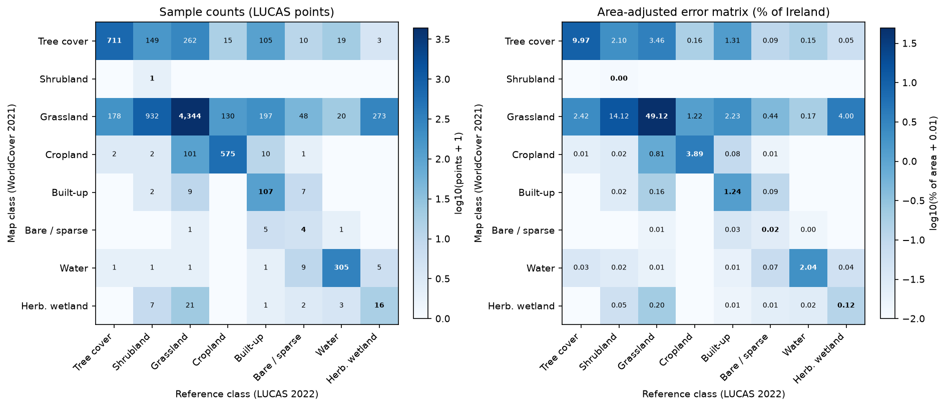
The right-hand matrix says something the counts hide. The single largest error in the map, at an estimated 14.1% of Ireland, is heath and scrub that WorldCover labels as grassland. Bog mapped as grassland adds another 4.0%.
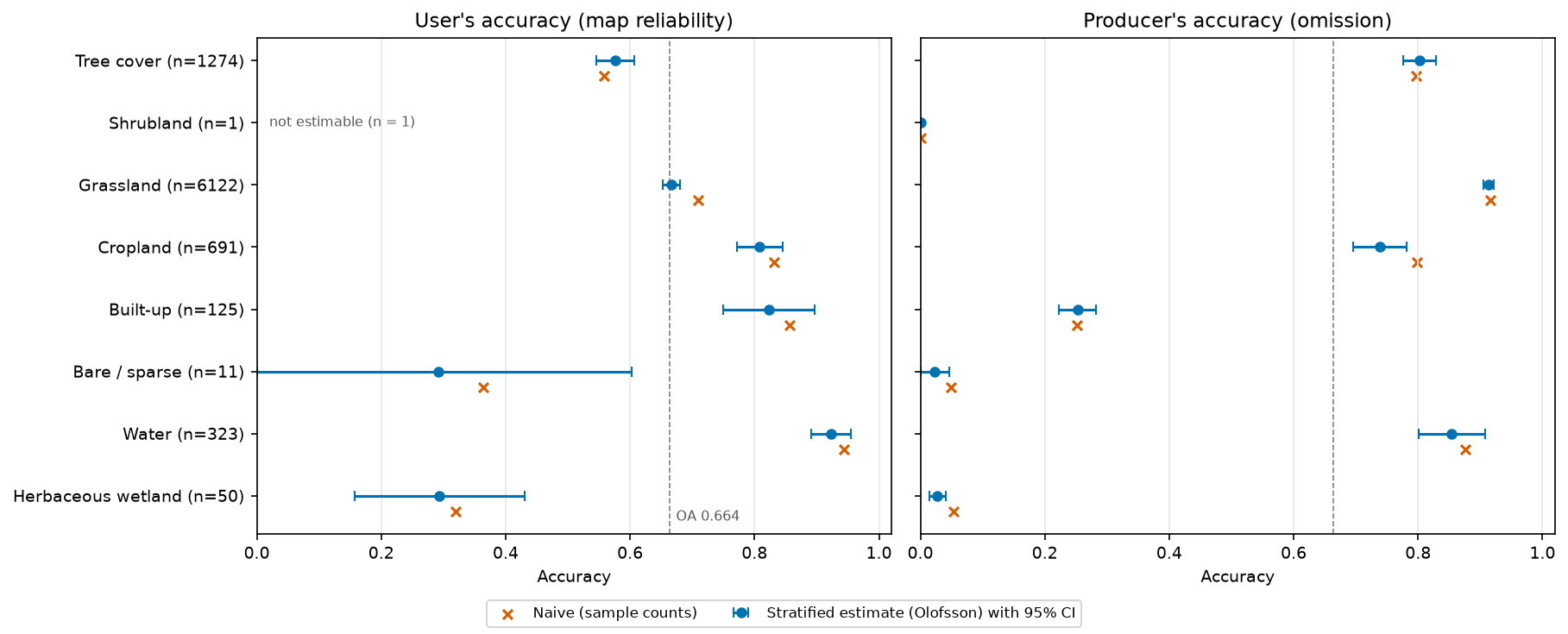
             class    n  n_eff UA_naive    UA UA_ci PA_naive    PA PA_ci map_km2 adj_km2 adj_ci_km2 boot_ci_km2 unweighted_km2        Tree cover 1274    989    0.558 0.576 0.031    0.797 0.803 0.027  12,095   8,687        463         438          8,264         Shrubland    1      1    1.000 1.000 0.000    0.001 0.000 0.000       1  11,417        654         607          9,335         Grassland 6122   4329    0.710 0.666 0.014    0.917 0.914 0.008  51,557  37,597        797         761         39,764          Cropland  691    448    0.832 0.808 0.036    0.799 0.739 0.043   3,370   3,687        242         225          4,042          Built-up  125    104    0.856 0.823 0.074    0.251 0.253 0.030   1,055   3,430        342         276          3,635     Bare / sparse   11      9    0.364 0.292 0.311    0.049 0.022 0.024      39     506        144         121            631             Water  323    270    0.944 0.923 0.032    0.876 0.854 0.054   1,546   1,671        115         103          1,829Herbaceous wetland   50     44    0.320 0.294 0.137    0.054 0.028 0.013     277   2,946        353         337          2,440
overall accuracy (area-weighted, design-weighted): 0.664 +/- 0.012 (bootstrap +/- 0.011); ignoring the design weights: 0.695; naive count-based: 0.705Pontius & Millones: quantity disagreement 0.248, allocation disagreement 0.088 (total 0.336); kappa on the area-adjusted matrix 0.419note: map shrubland has n = 1 point, so its user's accuracy is not estimable
The UA_ci, PA_ci and adj_ci_km2 columns are 95% confidence half-widths (1.96 × SE). Reading the table:
- Overall accuracy is 0.664 ± 0.012, not the 0.705 you get by counting agreeing points. The naive figure is inflated because LUCAS over-samples cropland and water, which WorldCover maps well. Ignoring the design weights but keeping the area weighting gives 0.695, so both corrections matter.
- User’s accuracy is high for water (0.923 ± 0.032), built-up (0.823 ± 0.074) and cropland (0.808 ± 0.036). Where WorldCover says built-up, it is usually right. It is low for tree cover (0.576 ± 0.031): many “tree” pixels are probably hedgerows, scrub or field edges, which LUCAS records as shrubland, grassland or tracks.
- Producer’s accuracy shows what the map misses. Only 25.3% of built-up land and 2.8% of herbaceous wetland end up in those classes on the map. Shrubland’s producer’s accuracy is effectively zero.
- Error-adjusted areas change the story. Grassland falls from 51,557 km² on the map to 37,597 ± 797 km². Shrubland rises from 1 km² to 11,417 ± 654 km², and herbaceous wetland from 277 km² to 2,946 ± 353 km². Built-up land is about three times its mapped area once roads and tracks are counted, at 3,430 ± 342 km². The bootstrap intervals (
boot_ci_km2) are close to the analytical ones throughout. - Quantity disagreement (0.248) is much larger than allocation disagreement (0.088). Most of the error comes from the map having the wrong amount of each class, which is exactly what error-adjusted area estimation corrects.
Step 8: caveats you can measure
Three mismatches between LUCAS and WorldCover could bias the result: what the point represents, how it was observed, and when.
def group_oa(mask):    return estimate(m[mask], r[mask], w[mask], W, K)[1], int(mask.sum())

sens = []ot = pts.SURVEY_OBS_TYPE.to_numpy()for k, label in [(1, "Field, <= 100 m"), (2, "Field, > 100 m"), (3, "PI in the field"), (7, "PI in the office")]: sens.append(("Observation type", label, *group_oa(ot == k)))pure = pts.pure3x3.to_numpy()sens.append(("3x3 map window", "All 9 pixels agree", *group_oa(pure == 1)))sens.append(("3x3 map window", "Mixed", *group_oa(pure < 1)))ext = pts[["SURVEY_CPRN_LC1N", "SURVEY_CPRNC_LC1E", "SURVEY_CPRNC_LC1S", "SURVEY_CPRNC_LC1W"]].min(1).to_numpy()cop = ~np.isnan(ext)sens.append(("Copernicus module", "Same cover >= 20 m all round", *group_oa(cop & (ext >= 20))))sens.append(("Copernicus module", "Same cover < 20 m", *group_oa(cop & (ext < 20)))) group subset OA n Observation type Field, <= 100 m 0.719 3933 Observation type Field, > 100 m 0.808 205 Observation type PI in the field 0.750 161 Observation type PI in the office 0.604 4298 3x3 map window All 9 pixels agree 0.699 7433 3x3 map window Mixed 0.489 1164Copernicus module Same cover >= 20 m all round 0.778 1041Copernicus module Same cover < 20 m 0.639 1624survey year: 2022 7,159, 2023 1,438 points (WorldCover 2021 describes 2021)map cropland, LUCAS grassland: 101 points, of which B55 temporary grassland 25LUCAS peat bog (H12) points by map class: Grassland 257, Herbaceous wetland 15, Water 2, Tree cover 1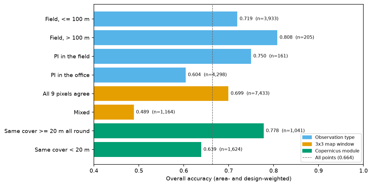
- Point vs pixel. A LUCAS point is a location, while a WorldCover pixel is a 10 m square, and both have positional error: GPS for the surveyor, and geolocation for Sentinel-2. Where the 3 × 3 map window is mixed, accuracy drops to 0.489; where it is uniform, it is 0.699. The LUCAS Copernicus module records how far the same cover extends in each direction. Where it reaches at least 20 m all round, accuracy is 0.778. Part of the “error” in the main estimate is therefore boundary and registration noise, not misclassification. You could restrict to homogeneous points, but that would no longer be a probability sample of Ireland, so report the full estimate and this sensitivity alongside it.
- Observation type. Half the Irish points (4,298) were photo-interpreted in the office, mostly remote upland and bog points that surveyors could not reach. They have the lowest accuracy (0.604). That reflects difficult landscapes as much as interpreter error, but treat the reference data as imperfect too.
- Date mismatch. WorldCover describes 2021, while LUCAS was surveyed from May 2022 to February 2023. Real change in one or two years is small for most classes, but rotations matter: 101 points mapped as cropland were grassland in LUCAS, and 25 of those were temporary grassland in a rotation.
- Bog and heath. Of 275 LUCAS peat bog points, WorldCover maps 257 as grassland and only 15 as herbaceous wetland. This is the single most important finding for Irish users: WorldCover does not separate bog and heath from grassland in Ireland.
Step 9: plan a new stratified random sample
If you are designing your own validation, the recommended design is a stratified random sample with the map classes as strata (Olofsson et al., 2014). Two questions: how many points in total, and how to split them between classes.
The total comes from Cochran’s (1977) formula for the standard error of overall accuracy under stratified sampling: n ≈ (Σ Wᵢ Sᵢ / SE)², where Sᵢ = √(Uᵢ(1 − Uᵢ)) and Uᵢ is a guess at each class’s user’s accuracy. This assessment provides those guesses. Where a class has fewer than 30 points, use 0.5, the worst case.
U_plan = np.where(n_i >= 30, np.clip(ua, 0.5, 0.95), 0.5)S = np.sqrt(U_plan * (1 - U_plan))target_se = 0.01n_total = int(np.ceil((np.sum(W * S) / target_se) ** 2))

def expected_se(n_alloc):    """Expected SE of OA and of each UA for an allocation, from the conjectured user's accuracies."""    v = U_plan * (1 - U_plan) / (np.maximum(n_alloc, 2) - 1)    return np.sqrt(np.sum(W ** 2 * v)), np.sqrt(v)

allocs = {}allocs["Proportional"] = np.maximum(np.round(n_total * W), 2)allocs["Equal"] = np.full(K, np.round(n_total / K))comp = np.full(K, 100.0) # at least 100 per class, the rest in proportion to arearest = n_total - comp.sum()big = W * n_total > 100comp[big] = np.round(100 + rest * W[big] / W[big].sum())allocs["Compromise (min 100)"] = compplanning user's accuracies: Tree cover 0.58, Shrubland 0.50, Grassland 0.67, Cropland 0.81, Built-up 0.82, Bare / sparse 0.50, Water 0.92, Herbaceous wetland 0.50Cochran (1977) eq. 5.25 with target SE(OA) = 0.01: n = 2171Proportional n = 2174: SE(OA) 0.0100; SE(UA) Tree 0.026, Shrubland 0.500, Grassland 0.012, Cropland 0.039, Built-up 0.067, Bare 0.500, Water 0.039, Herbaceous 0.177Equal n = 2168: SE(OA) 0.0218; SE(UA) Tree 0.030, Shrubland 0.030, Grassland 0.029, Cropland 0.024, Built-up 0.023, Bare 0.030, Water 0.016, Herbaceous 0.030Compromise (min 100) n = 2171: SE(OA) 0.0113; SE(UA) Tree 0.027, Shrubland 0.050, Grassland 0.014, Cropland 0.030, Built-up 0.038, Bare 0.050, Water 0.027, Herbaceous 0.050compromise allocation: Tree cover 347, Shrubland 100, Grassland 1155, Cropland 169, Built-up 100, Bare / sparse 100, Water 100, Herbaceous wetland 100wrote 2,171 stratified random sample points to output/worldcover_ireland_validation_sample.gpkg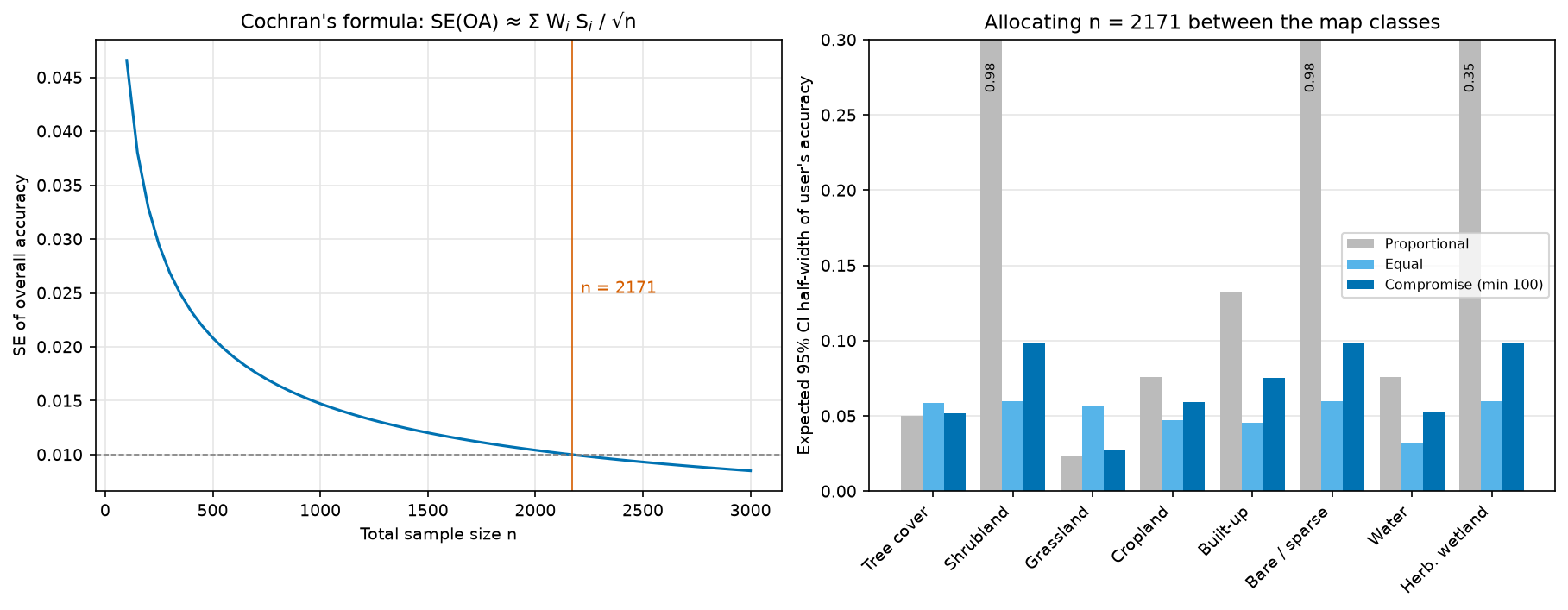
Proportional allocation meets the overall-accuracy target, but gives shrubland and bare land 2 points each, so their user’s accuracy cannot be estimated. Equal allocation estimates every class well but more than doubles the standard error of overall accuracy and the large-class areas. The compromise, at least 100 points per class with the rest in proportion to area, is what Olofsson et al. (2014) recommend in practice, and it costs only 0.0013 in SE(OA).
The script then draws that sample. It picks pixels at random within each map class without replacement, using the per-window class counts from Step 2 so it never has to load a whole tile. It shuffles the points so interpreters cannot guess the map class from the order, and writes a GeoPackage with an empty reference column for interpreters to fill in, blind to the map label. Feed their labels back into estimate() with all weights equal to 1, and you have a design-based assessment without any of the LUCAS caveats.
Limitations and honest caveats
- The reference is not truth. LUCAS is excellent but not perfect: about half the Irish points are office photo-interpretations, and the LUCAS legend was not designed for WorldCover. The estimates measure agreement with LUCAS through this crosswalk.
- Post-stratification is approximate. The estimators treat LUCAS as a stratified sample by map class, with design-weighted proportions within each class. Variances use Kish’s effective sample size and ignore the systematic grid and the second-phase stratification. The stratified bootstrap gives very similar intervals, which is reassuring but not proof.
- Rare map classes are barely sampled. WorldCover shrubland has one point and bare land eleven, so their user’s accuracies are not estimable or are very uncertain. A map-stratified design (Step 9) fixes this.
- Point-vs-pixel and registration error lower measured accuracy, by roughly 0.2 at mixed pixels. The main estimate includes them on purpose, because that is the accuracy a user experiences at a random location.
- The time mismatch is one to two years. That is small for forests and water, but not for crop rotations.
- One country. WorldCover’s accuracy varies by biome. Irish heath and bog are a known weak spot, so don’t extrapolate these numbers to other countries.
Frequently asked questions
What is the difference between user’s accuracy and producer’s accuracy?
User’s accuracy answers the map user’s question: if the map says forest here, how likely is it to be forest? It is calculated along the rows (map classes) and is one minus the commission error. Producer’s accuracy answers the map-maker’s question: of all the real forest, how much did the map capture? It is calculated down the columns (reference classes) and is one minus the omission error. A class can score high on one and low on the other. Built-up land in Ireland has a user’s accuracy of 0.82 but a producer’s accuracy of 0.25.
Why is the kappa coefficient no longer recommended?
Kappa measures agreement relative to a hypothetical random allocation of the map’s own class proportions. That baseline is irrelevant to whether the map is useful, and the resulting index is hard to interpret and can rank maps inconsistently (Pontius and Millones, 2011). Good-practice guidance (Olofsson et al., 2014) recommends reporting overall, user’s and producer’s accuracy with confidence intervals. If you need to decompose the error, report quantity and allocation disagreement instead.
How do I calculate error-adjusted area from a confusion matrix?
Convert each row of the count matrix to proportions, and multiply by that map class’s share of the mapped area, Wᵢ. The column sums of the result are the estimated true area proportions; multiply by the total area to get km². The standard error of each area is √(Σᵢ Wᵢ² pᵢⱼ(1 − pᵢⱼ)/(nᵢ − 1)) times the total area, and the 95% confidence interval is ±1.96 SE (Olofsson et al., 2014, equations 9–11). This only works if your sample is a probability sample with known inclusion probabilities.
How many sample points do I need for an accuracy assessment?
Use Cochran’s formula for stratified sampling, n = (Σ Wᵢ Sᵢ / SE)², with Sᵢ = √(Uᵢ(1 − Uᵢ)) based on your best guess of each class’s user’s accuracy and a target standard error for overall accuracy. A target SE of 0.01 needed 2,171 points for WorldCover in Ireland. Then allocate at least 50–100 points to every class, and spread the rest in proportion to area, so that rare classes get a usable user’s accuracy.
Can I use existing survey data like LUCAS instead of collecting my own reference sample?
Yes, if it is a probability sample and you can recover each point’s selection probability, as you can for LUCAS from the master grid. Weight each point by the inverse of that probability and post-stratify by the map classes. Check the legend crosswalk, the observation date and the point-vs-pixel support, and report them. If the survey was not a probability sample (for example, opportunistic field visits), you cannot make unbiased area or accuracy estimates from it.
Does stratified random sampling bias the overall accuracy?
Not if you analyse it with the stratified estimators. Sampling rare classes more heavily changes the precision, not the expected value, because each map class is weighted by its mapped area when the results are combined. Bias comes from analysing a stratified sample as if it were simple random: here that gave 0.705 instead of 0.664.
Next steps
- Produce your own map with the random forest land cover classification tutorial, then assess it with a held-out probability sample rather than its training data.
- The habitat mapping series builds a finer-grained habitat map. The same estimators work, but you will need more points per class.
- If your map comes with a time dimension, the Mann-Kendall raster trend analysis tutorial is a companion piece on testing many pixels at once, including false discovery rate control.
- For spatial clustering of errors, the hot spot analysis tutorial shows how to test whether disagreement points are clustered.
Data and licences
- ESA WorldCover 2021 v200: © ESA WorldCover project 2021 / Contains modified Copernicus Sentinel data (2021) processed by the ESA WorldCover consortium. Licensed under CC BY 4.0. Tiles are read from the ESA WorldCover AWS bucket.
- LUCAS 2022 microdata and master grid: © European Union, Eurostat. Reuse is authorised with acknowledgement of the source. See the Eurostat LUCAS pages.
- NUTS 2021 boundaries: © EuroGeographics for the administrative boundaries, distributed by Eurostat GISCO.
References: Olofsson, P., Foody, G. M., Herold, M., Stehman, S. V., Woodcock, C. E. and Wulder, M. A. (2014) “Good practices for estimating area and assessing accuracy of land change”, Remote Sensing of Environment, 148, 42–57. Pontius, R. G. and Millones, M. (2011) “Death to Kappa”, International Journal of Remote Sensing, 32(15), 4407–4429. Cochran, W. G. (1977) Sampling Techniques, 3rd edn. Wiley.
The full script is accuracy_assessment.py. It was tested on Python 3.12.0 with numpy 2.5.4, pandas 3.1.0, geopandas 1.2.0, rasterio 1.5.2, shapely 2.2.0, pyproj 3.8.0 and matplotlib 3.11.2 on 27 October 2026.
Key terms
- Confusion matrix (error matrix)
- A table that cross-tabulates map labels (rows here) against reference labels (columns) at sample locations. The diagonal holds agreement; everything off the diagonal is an error.
- Overall accuracy
- The proportion of the mapped area that is correctly classified: the sum of the diagonal of the area-proportion error matrix.
- User's accuracy
- For a map class, the proportion of its mapped area that really is that class. One minus user's accuracy is the commission error.
- Producer's accuracy
- For a reference class, the proportion of its true area that the map labels correctly. One minus producer's accuracy is the omission error.
- Stratified estimator
- An estimator that combines per-stratum sample results with the known size of each stratum. Here the strata are the map classes and their sizes are the mapped areas.
- Error-adjusted area
- An estimate of the true area of each class: the column total of the area-proportion error matrix times the total area. It corrects the bias of pixel counting.
- Post-stratification
- Treating a sample that was not stratified by the map as if it had been, by grouping points by map class after selection and weighting each group by its mapped area.
- Quantity and allocation disagreement
- Pontius and Millones's split of total map error into a part caused by wrong class proportions (quantity) and a part caused by wrong locations (allocation).
Data for this tutorial
- ESA WorldCover · The 10 m global land cover map assessed here (2021, v200), read as Cloud Optimised GeoTIFFs from AWS
- Eurostat LUCAS · The 2022 field survey points and master grid used as reference data
- Eurostat GISCO · NUTS 2021 boundaries used for the Ireland study area
- National Land Cover Map (Ireland) · Ireland's national high-resolution land cover map: a better-detailed map to assess the same way
Licences and formats for each source are listed in the GIS data sources catalogue.