Cloud Optimised GeoTIFFs in Python: reproject, mosaic and validate a COG

Short answer: to create a Cloud Optimised GeoTIFF in Python, write your raster as usual and convert it with rio-cogeo: cog_translate("in.tif", "out.tif", cog_profiles.get("deflate"), overview_resampling="average"), then check it with cog_validate("out.tif"). With rasterio alone, rasterio.shutil.copy("in.tif", "out.tif", driver="COG", COMPRESS="DEFLATE", PREDICTOR="YES", BLOCKSIZE=512) does the same through GDAL’s COG driver. To reproject and mosaic first, open the source tiles (they can be https:// URLs), combine them with rasterio.merge.merge, and warp the result with rasterio.warp.reproject.

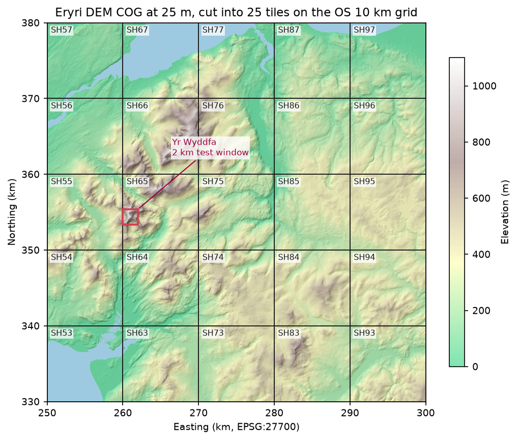
This is part 1 of the two-part series Cloud-native rasters in Python. We mosaic four Copernicus DEM tiles straight from Amazon S3, reproject them to British National Grid, and write a validated COG of Eryri (Snowdonia). Along the way we count every byte that GDAL fetches, so you can see what “cloud-native” buys you. Finally we cut the COG into 25 tiles on the Ordnance Survey 10 km grid. In part 2, those tiles become a static STAC catalogue built with pystac, which we validate, query and compare with the Earth Search and Planetary Computer STAC APIs.

You will learn how to:

1. read remote COGs with rasterio, and count the HTTP range requests behind each read;
2. mosaic several tiles with rasterio.merge and reproject them to a projected grid;
3. write a COG with rio-cogeo and with the GDAL COG driver, and validate it;
4. see the internal tiles and overviews inside the file;
5. choose the compression, predictor and block size, with measured sizes;
6. serve your own COG over HTTP and measure what windowed and overview reads cost.

All outputs below are real results from cog_mosaic.py, run on 3 November 2026 on Windows 11 from the UK with Python 3.12.0, rasterio 1.5.2 (GDAL 3.12.2), rio-cogeo 7.0.4, numpy 2.5.4 and pandas 3.1.0.

Set up

pip install rasterio==1.5.2 rio-cogeo==7.0.4 numpy==2.5.4 pandas==3.1.0 matplotlib==3.11.2 pyproj==3.8.0 requests==2.34.2

The rasterio wheels bundle GDAL, so you need nothing else. The Copernicus tiles sit in the public AWS bucket copernicus-dem-30m and need no account or credentials. Each 1 x 1 degree tile has a predictable URL:

TILES = ["N53_00_W005_00", "N53_00_W004_00", "N52_00_W005_00", "N52_00_W004_00"]
BUCKET = "https://copernicus-dem-30m.s3.amazonaws.com"
BNG = "EPSG:27700"
AOI = (250_000, 330_000, 300_000, 380_000)   # 50 x 50 km of Eryri in British National Grid (OS square SH)
RES = 25                                      # output pixel size in metres: 10 km = 400 pixels exactly


def tile_url(tile: str) -> str:
    name = f"Copernicus_DSM_COG_10_{tile}_DEM"
    return f"{BUCKET}/{name}/{name}.tif"

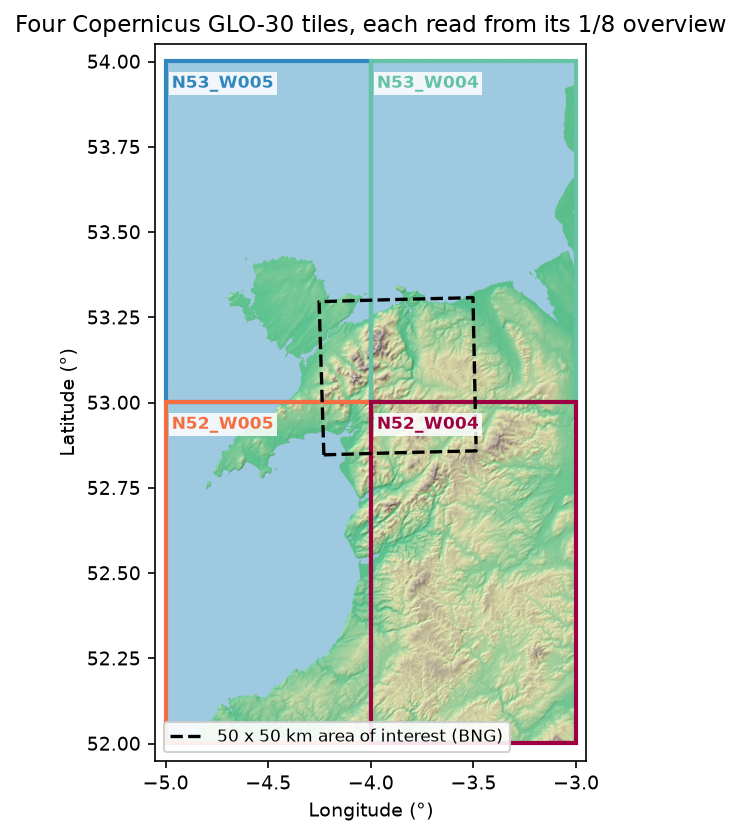
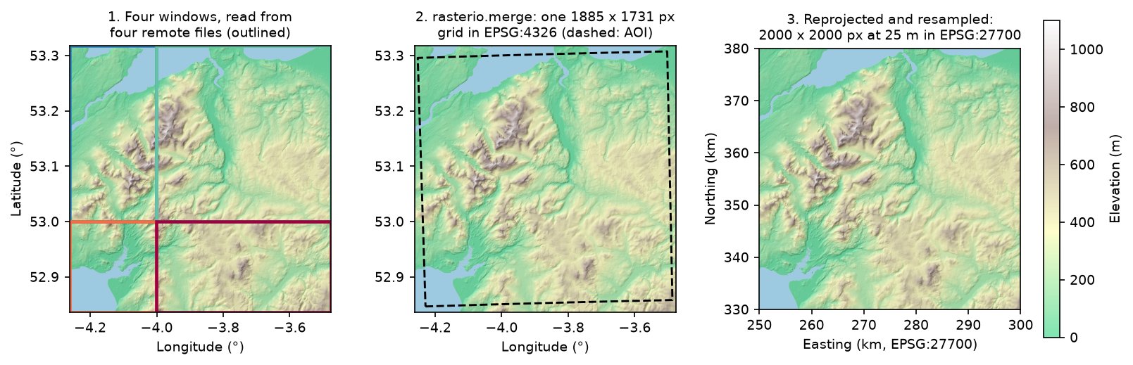
Our area of interest is the 50 x 50 km square from easting 250 km to 300 km and northing 330 km to 380 km, which covers Yr Wyddfa (Snowdon), the Glyderau, the Carneddau and the Conwy valley. In longitude and latitude it straddles the corner where four GLO-30 tiles meet.

Counting the bytes GDAL fetches

GDAL reads remote files through its /vsicurl/ layer, which turns each read into HTTP range requests. With CPL_DEBUG on, it logs every request as Downloading 0-16383 ..., and rasterio passes those messages to Python’s logging. A small handler adds them up:

RANGES: list[tuple[int, int]] = []


class RangeLog(logging.Handler):
    def emit(self, record):
        for a, b in re.findall(r"Downloading (\d+)-(\d+)", record.getMessage()):
            RANGES.append((int(a), int(b)))


logging.getLogger("rasterio").addHandler(RangeLog())
GDAL_ENV = dict(GDAL_DISABLE_READDIR_ON_OPEN="EMPTY_DIR", CPL_VSIL_CURL_ALLOWED_EXTENSIONS=".tif")

The two GDAL settings matter for any remote read. GDAL_DISABLE_READDIR_ON_OPEN="EMPTY_DIR" stops GDAL listing the “directory” on S3 to look for sidecar files, and CPL_VSIL_CURL_ALLOWED_EXTENSIONS stops it probing for .aux.xml and .ovr files that don’t exist. The script’s measured() helper switches debug logging on, runs a read inside rasterio.Env(CPL_DEBUG=True, **GDAL_ENV), and returns the median time of three runs with the request and byte counts. A unique ?run=N query string on each URL stops GDAL’s in-process cache from answering a repeat read.

Step 1: inspect the source COGs

Opening a COG reads only its header, so we can inspect all four tiles and read a 1/8-resolution preview of each from its overviews:

with rasterio.open(url) as src:
    print(src.width, src.height, src.block_shapes, src.overviews(1), src.compression, src.nodata)
    arr = src.read(1, out_shape=(src.height // 8, src.width // 8))   # served from the 1/8 overview

          tile     size_px    blocks overviews compress predictor  file_MB  thumb_requests  thumb_MB
N53_00_W005_00 2400 x 3600 1024x1024 [2, 4, 8]  DEFLATE         3      5.8               2      0.10
N53_00_W004_00 2400 x 3600 1024x1024 [2, 4, 8]  DEFLATE         3     11.4               2      0.18
N52_00_W005_00 2400 x 3600 1024x1024 [2, 4, 8]  DEFLATE         3     10.1               2      0.16
N52_00_W004_00 2400 x 3600 1024x1024 [2, 4, 8]  DEFLATE         3     30.9               2      0.43
crs: EPSG:4326 | pixel size (deg): (0.0004167, 0.0002778) | nodata: None
AOI in BNG: (250000, 330000, 300000, 380000) -> lon/lat bounds: (-4.2521, 52.8466, -3.4867, 53.3075)

Each tile is already a COG: 1024 px blocks, overviews at 1/2, 1/4 and 1/8, DEFLATE with the floating-point predictor. Each preview cost two requests and 0.10–0.43 MB, between 1.4% and 1.7% of each file. Above 50° N, GLO-30 tiles are 2400 pixels wide, not 3600: the longitude spacing widens to 1.5 arc-seconds so that pixels stay roughly square on the ground. The tile sizes vary sixfold because sea compresses to almost nothing, while the hills of N52_W004 do not.

Step 2: a windowed read against the whole file

The largest tile, N52_W004, holds Arenig Fawr and the hills around Bala. We read a 5 km window at full resolution, the whole tile through rasterio, and the whole file with requests.get, three times each:

def window_read():
    with rasterio.open(fresh(big)) as src:
        return src.read(1, window=from_bounds(*win_ll, transform=src.transform))

tile N52_00_W004_00: 30.9 MB on S3 (eu-central-1); median of 3 runs
                               job      pixels  requests     MB  pct_of_file  seconds
                 open: header only           -         1  0.016        0.053    0.086
      5 km window, full resolution   192 x 180         2  2.753        8.909    0.241
           whole tile via rasterio 2400 x 3600         4 22.820       73.857    1.543
download whole file (requests.get)           -         1 30.897      100.000    2.039

• Opening is one 16 kB request. GDAL reads the first 16 kB, which holds the header and the offsets of every block, and stops.
• The window cost 8.9% of the file. The 192 x 180 px window sits inside one 1024 px block, so GDAL fetched just that block’s compressed bytes: 2.75 MB in one extra request.
• Even the whole tile at full resolution skipped 26% of the file. Those bytes are the overviews, which a full-resolution read never needs. GDAL also merges neighbouring blocks into a few large requests, so the whole tile took four requests, not 12.

Step 7 below repeats this on our own files, and Figure 5 charts both.

Step 3: mosaic and reproject

rasterio.merge.merge accepts a list of paths or URLs and a target bounding box, and reads only the windows that it needs from each source:

from rasterio.merge import merge
from rasterio.warp import reproject

pad = 0.01
read_bounds = (aoi_ll[0] - pad, aoi_ll[1] - pad, aoi_ll[2] + pad, aoi_ll[3] + pad)
mosaic_ll, ll_transform = merge([tile_url(t) for t in TILES], bounds=read_bounds, resampling=Resampling.nearest)
mosaic_ll = mosaic_ll[0]

width = height = int((AOI[2] - AOI[0]) / RES)
dst_transform = from_origin(AOI[0], AOI[3], RES, RES)
dem = np.full((height, width), np.nan, dtype="float32")
reproject(mosaic_ll, dem, src_transform=ll_transform, src_crs="EPSG:4326", dst_transform=dst_transform,
          dst_crs=BNG, resampling=Resampling.bilinear, dst_nodata=np.nan)

rasterio.merge: 1885 x 1731 px in EPSG:4326 from 4 remote tiles, 10 range requests, 17.86 MB, 1.6 s
  N53_00_W005_00: window 629 x 1142 px
  N53_00_W004_00: window 1257 x 1142 px
  N52_00_W005_00: window 629 x 589 px
  N52_00_W004_00: window 1257 x 589 px
reprojected to EPSG:27700 at 25 m: 2000 x 2000 px in 0.19 s; NaN pixels: 0
elevation min/mean/max (m): -1.7 / 264.6 / 1071.8; sea and lakes at 0 m or below: 6.2%

The four tiles hold 58.2 MB between them; the mosaic needed 17.86 MB. We pad the bounding box by 0.01° (about 700 m) so that the reprojected square never runs off the edge of the mosaic; the zero NaN count confirms it. We use nearest resampling to merge, because the tiles share one grid and no values need to change. We use bilinear to reproject, because the British National Grid pixels don’t line up with the source pixels.

Step 4: write the COG, and compare the options

First we write the DEM as a plain GeoTIFF with GDAL’s defaults, then convert it with rio-cogeo:

from rio_cogeo.cogeo import cog_translate, cog_validate
from rio_cogeo.profiles import cog_profiles

with rasterio.open("eryri_dem_25m_plain.tif", "w", driver="GTiff", dtype="float32", count=1, width=width,
                   height=height, crs=BNG, transform=dst_transform) as dst:
    dst.write(dem, 1)

cog_profile = cog_profiles.get("deflate")
cog_profile.update(predictor=3, blockxsize=512, blockysize=512)
cog_translate("eryri_dem_25m_plain.tif", "eryri_dem_25m_cog.tif", cog_profile, overview_resampling="average",
              additional_cog_metadata={"SOURCE": "Copernicus DEM GLO-30 (AWS copernicus-dem-30m), 4 tiles"})
print(cog_validate("eryri_dem_25m_cog.tif"))

plain GeoTIFF (GDAL defaults): 16.02 MB, valid COG: False
rio-cogeo COG: 13.19 MB in 0.85 s; valid COG: True; errors: []; warnings: []

cog_validate returns a tuple of (is_valid, errors, warnings). The plain GeoTIFF fails because GDAL writes uncompressed strips by default, with no overviews. Use average resampling for the overviews of continuous data such as elevation; the default, nearest, picks one pixel in each block and makes the overviews noisy.

GDAL 3.1 and later also has a dedicated COG driver, which you can call through rasterio.shutil.copy. We used it to write six variants of the same DEM:

rasterio.shutil.copy("eryri_dem_25m_plain.tif", "eryri_dem_25m_zstd.tif", driver="COG", BLOCKSIZE=512,
                     COMPRESS="ZSTD", PREDICTOR="YES", OVERVIEW_RESAMPLING="AVERAGE")

                   variant  block     MB  write_s  valid overviews  max_abs_error_m
     DEFLATE, no predictor    512 17.070    0.844   True    [2, 4]              0.0
       DEFLATE + predictor    512 13.194    0.776   True    [2, 4]              0.0
          ZSTD + predictor    512 12.907    0.585   True    [2, 4]              0.0
LERC_ZSTD, max error 0.1 m    512  5.299    0.277   True    [2, 4]              0.1
       DEFLATE + predictor    256 13.383    0.814   True [2, 4, 8]              0.0
       DEFLATE + predictor   1024 12.496    0.702   True       [2]              0.0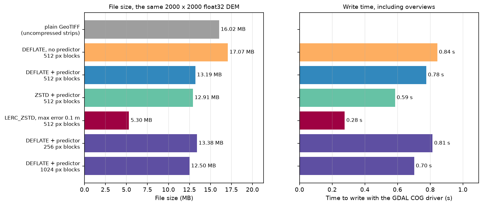

What the numbers show:

• Use the predictor for float data. The raw bytes of float32 elevations look almost random to DEFLATE. PREDICTOR=YES (which the COG driver turns into the floating-point predictor, 3, for float data) stores differences between neighbours instead, and saved 23%.
• ZSTD is slightly smaller and faster than DEFLATE, but older GDAL builds (before 2.3) and some non-GDAL readers can’t decode it. DEFLATE is the safe default for files you publish.
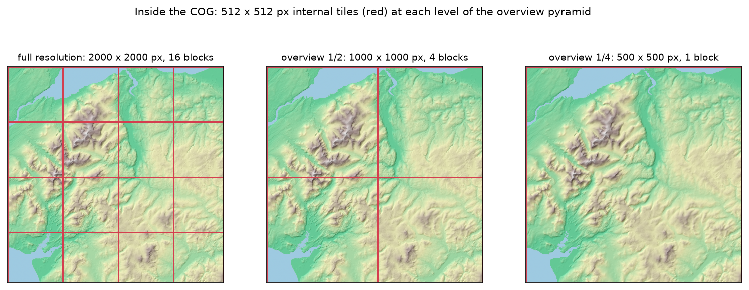
• LERC is lossy, and honest about it. MAX_Z_ERROR=0.1 guarantees every pixel within 0.1 m of the original, which the script confirms. For a 30 m DSM whose own vertical accuracy is metres, that loss is negligible, and the file is 60% smaller.
• The block size sets the number of overviews. The COG driver adds overviews until the smallest one fits in a single block: 2000 → 1000 → 500 px with 512 px blocks, one level fewer with 1024 px, one more with 256 px. Step 7 shows why that matters.

Step 5: look inside the COG

cog_info lists every image file directory (IFD), with its size and block shape:

from rio_cogeo.cogeo import cog_info

info = cog_info("eryri_dem_25m_cog.tif")
for ifd in info.IFD:
    print(ifd.Level, ifd.Width, ifd.Height, ifd.Blocksize, ifd.Decimation)

compression: DEFLATE | COG layout: COG | predictor: 3
  IFD level 0: 2000 x 2000 px, blocks 512 x 512, decimation 0
  IFD level 1: 1000 x 1000 px, blocks 512 x 512, decimation 2
  IFD level 2: 500 x 500 px, blocks 512 x 512, decimation 4

The LAYOUT=COG tag tells readers that the file follows the COG layout: all IFDs at the front, then the overview blocks from smallest to largest, then the full-resolution blocks. A reader that only wants a preview finds the small overview near the start of the file.

Step 6: cut 25 COG tiles on the OS 10 km grid

Part 2 needs a set of files to catalogue, so we cut the COG into the 25 Ordnance Survey 10 km squares it covers. A 10 km square is 400 pixels, so each window lines up exactly:

with rasterio.open("eryri_dem_25m_cog.tif") as src:
    for e in range(AOI[0], AOI[2], 10_000):
        for n in range(AOI[1], AOI[3], 10_000):
            name = f"SH{(e % 100_000) // 10_000}{(n % 100_000) // 10_000}"     # e.g. SH65 contains Yr Wyddfa
            w = from_bounds(e, n, e + 10_000, n + 10_000, transform=src.transform).round_offsets().round_lengths()
            arr = src.read(1, window=w)
            # write arr to a temporary GeoTIFF, then:
            rasterio.shutil.copy(tmp, TILE_DIR / f"{name}.tif", driver="COG", BLOCKSIZE=256,
                                 COMPRESS="DEFLATE", PREDICTOR="YES", OVERVIEW_RESAMPLING="AVERAGE")

25 tiles of 400 x 400 px, all valid COGs: True, total 12.72 MB
tile  valid    kB  min_m  max_m
SH65   True 537.8   53.6 1071.8
SH66   True 521.6   33.0 1059.2
SH76   True 549.8    1.0  875.1
SH75   True 546.4    8.2  865.0
SH83   True 508.7  158.5  846.5

For 400 px tiles, 256 px blocks keep the internal tiling useful; with 512 px blocks, each tile would be a single block. The two letters and two digits are the standard OS grid reference: SH65 is the square whose south-west corner is at easting 260 km and northing 350 km, and it contains Yr Wyddfa.

Step 7: range reads from our own files

To measure our own files, the script serves its output/ folder on localhost with a 30-line subclass of http.server.SimpleHTTPRequestHandler. Python’s built-in server ignores Range headers, so the subclass answers them with 206 Partial Content and records the bytes it sends. We then read three things from four files: a 2 x 2 km window around Yr Wyddfa, the whole area at 1/16 resolution, and the whole file.

with rasterio.Env(**GDAL_ENV), rasterio.open(f"/vsicurl/{base}/{path.name}") as s:
    win = s.read(1, window=from_bounds(*snow_win, transform=s.transform))     # 2 x 2 km
    ovr = s.read(1, out_shape=(s.height // 16, s.width // 16))              # 1/16 resolution

              file                           job      pixels  requests     MB  pct_of_file       ms
     plain GeoTIFF  2 x 2 km window at Yr Wyddfa     80 x 80         4  0.689        4.302   12.000
     plain GeoTIFF whole area at 1/16 resolution   125 x 125         5 15.976       99.693 1085.806
     plain GeoTIFF   whole file, full resolution 2000 x 2000         5 16.025      100.000 1006.250
 COG 512 px blocks  2 x 2 km window at Yr Wyddfa     80 x 80         3  1.393       10.555   18.332
 COG 512 px blocks whole area at 1/16 resolution   125 x 125         2  0.721        5.464   12.887
 COG 512 px blocks   whole file, full resolution 2000 x 2000         2  9.868       74.793  866.849
 COG 256 px blocks  2 x 2 km window at Yr Wyddfa     80 x 80         3  0.359        2.681   10.762
 COG 256 px blocks whole area at 1/16 resolution   125 x 125         2  0.197        1.469    8.490
 COG 256 px blocks   whole file, full resolution 2000 x 2000         2  9.860       73.678  812.067
COG 1024 px blocks  2 x 2 km window at Yr Wyddfa     80 x 80         3  4.922       39.385  128.039
COG 1024 px blocks whole area at 1/16 resolution   125 x 125         2  2.654       21.240   88.044
COG 1024 px blocks   whole file, full resolution 2000 x 2000         2  9.875       79.022  810.774
highest pixel within 1 km of Yr Wyddfa: 1071.8 m (published summit height 1,085 m)
highest native GLO-30 pixel in the same area: 1074.5 m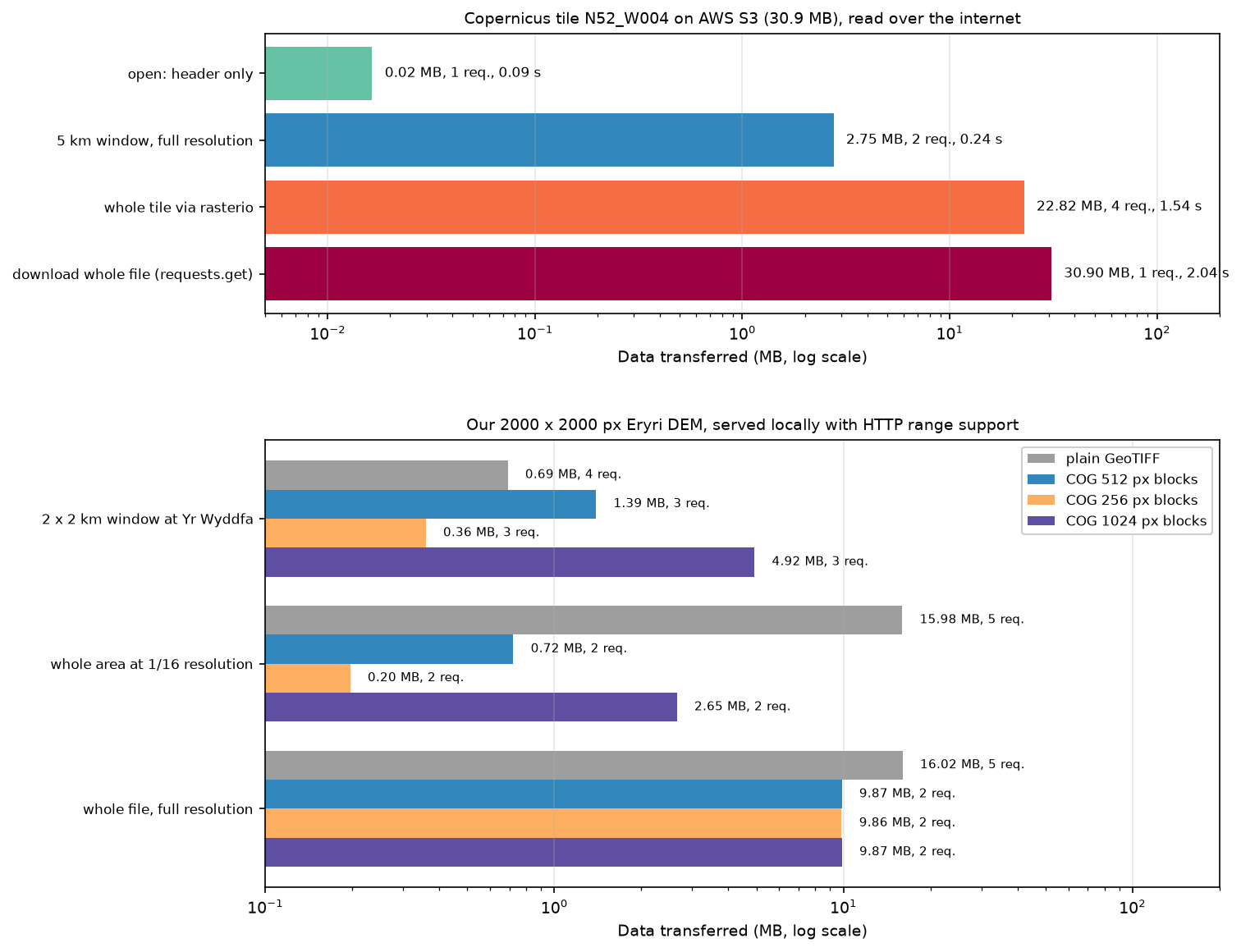

• Overviews are the big win. The plain GeoTIFF had to send 99.7% of itself for a 125 x 125 px preview, because GDAL had to read every pixel to average them. The 512 px COG sent 0.72 MB from its 1/4 overview.
• Small blocks favour small windows. The 80 x 80 px window crosses a block boundary, so it needed two blocks: 0.36 MB with 256 px blocks, 1.39 MB with 512 px and 4.92 MB with 1024 px. Larger blocks compress slightly better (Step 4) and need fewer requests for big reads. 512 px is a balanced default; choose 256 px when users mostly zoom in on small areas.
• The plain GeoTIFF won the small window. Its uncompressed strips are full-width rows, and 80 rows of 2000 float32 pixels are only 0.64 MB. That advantage disappears as soon as the data is compressed or you want a preview.
• Whole-file reads skip the overviews. Every COG read 74–79% of itself for the full-resolution grid.

The localhost timings show the CPU cost of decompressing, not network latency. Over the internet, as in Step 2, each request also costs a round trip, which is why GDAL merges neighbouring blocks into one request.

The summit check is a useful sanity test. The highest pixel near Yr Wyddfa is 1071.8 m, against the published 1,085 m. The native GLO-30 pixels reach 1074.5 m: a 30 m pixel averages the summit with the slopes around it, and bilinear resampling to 25 m smooths it a little further.

Limitations and caveats

• GLO-30 is a surface model. It includes trees and buildings, and its heights refer to the EGM2008 geoid, not Ordnance Datum Newlyn, the datum of Ordnance Survey heights. Check the offset before you compare it with OS spot heights or surveys.
• No nodata value. The tiles have no nodata, and the sea is stored as 0 m or just below (6.2% of our grid). To mask the sea reliably, use a coastline polygon rather than an elevation threshold.
• Timings vary. Step 2 used one home connection to the eu-central-1 region; Step 7 used localhost. Byte and request counts are the reliable figures, and they were identical across repeated runs.
• GDAL’s request merging changes with settings. GDAL_HTTP_MERGE_CONSECUTIVE_RANGES and CPL_VSIL_CURL_CHUNK_SIZE (16 kB by default) change how reads are split. Our counts use GDAL 3.12.2 defaults.
• COG is a layout, not a guarantee. A valid COG with huge blocks or no overviews still reads badly. Always check block size and overviews, as cog_info shows.

Frequently asked questions

How do I create a Cloud Optimized GeoTIFF in Python?

Use rio-cogeo: cog_translate(src_path, dst_path, cog_profiles.get("deflate"), overview_resampling="average"), then cog_validate(dst_path). Or use rasterio with GDAL’s COG driver: rasterio.shutil.copy(src_path, dst_path, driver="COG", COMPRESS="DEFLATE", PREDICTOR="YES"). Both write internal tiles, overviews and the COG layout in one step. The command-line equivalent is gdal_translate in.tif out.tif -of COG -co COMPRESS=DEFLATE -co PREDICTOR=YES.

How do I reproject and mosaic rasters with rasterio?

Pass the files or URLs to rasterio.merge.merge(paths, bounds=...) to get one array and its transform, then call rasterio.warp.reproject with the source and destination transforms and CRSs. Pad the bounds slightly so that the reprojected grid stays inside the mosaic. For large areas, rasterio.vrt.WarpedVRT or a GDAL VRT avoids holding the whole mosaic in memory.

What is the difference between a GeoTIFF and a COG?

A COG is a GeoTIFF with a specific internal layout: tiled rather than striped, with overviews, and with all the metadata at the front of the file. Any GeoTIFF reader can open it. Readers that understand HTTP range requests can also fetch just the parts they need, which here cut a preview read from 15.98 MB to 0.72 MB.

What block size and compression should I use for a COG?

For most rasters, use 512 px blocks with DEFLATE, plus PREDICTOR=YES for float data or PREDICTOR=2 for integers. Use 256 px blocks if people mostly read small windows, and ZSTD if every reader you care about runs GDAL 2.3 or later. For elevation where a known error bound is acceptable, LERC gave a file 60% smaller.

Can I read a COG from S3 without downloading it?

Yes. Pass the https:// URL (or s3:// with credentials) to rasterio.open and read a window. Rasterio uses GDAL’s /vsicurl/ layer, which fetches only the byte ranges it needs. Here a 5 km window from a 30.9 MB tile cost 2.75 MB and a quarter of a second.

Next steps

• Continue with part 2: build a STAC catalogue with pystac, which catalogues these 25 tiles, validates the catalogue, and compares it with the Earth Search and Planetary Computer STAC APIs.
• Compute slope, aspect and hillshade from this DEM in Raster terrain analysis with rasterio.
• Learn more about British National Grid and reprojection in Coordinate reference systems in Python.
• Use the COG for a viewshed analysis from Yr Wyddfa, or delineate the Conwy catchment.
• Print the mountain: DEM to STL in Python turns a tile into a 3D model.
• Turn classified rasters into polygons in Raster to vector in Python.

Data and licences

• Copernicus DEM GLO-30, tiles N52–N53, W004–W005, read from the AWS Open Data bucket copernicus-dem-30m. © DLR e.V. 2010–2014 and © Airbus Defence and Space GmbH 2014–2018, provided under COPERNICUS by the European Union and ESA; all rights reserved. GLO-30 is free to use, including commercially, under the Copernicus DEM licence; credit it as above.
• Code: cog_mosaic.py, tested with Python 3.12.0, rasterio 1.5.2 (GDAL 3.12.2), rio-cogeo 7.0.4, numpy 2.5.4, pandas 3.1.0, matplotlib 3.11.2, pyproj 3.8.0 and requests 2.34.2. Pinned versions are in requirements.txt.