Sentinel-1 soil moisture in Python: change detection checked against COSMOS-UK

Short answer: to estimate soil moisture from Sentinel-1 in Python, use change detection. Stream a long VV backscatter time series for each pixel from the Planetary Computer’s sentinel-1-rtc collection. Separately for each relative orbit, take a low percentile as the dry reference and a high percentile as the wet reference. Each date’s relative surface soil moisture is then (σ⁰ − dry) / (wet − dry) × 100 %. It is relative (0–100 %), it describes only the top few centimetres, and vegetation and surface roughness can overwhelm it, so check it against in-situ data before you trust it.

Wet soil reflects more microwave energy than dry soil, because water raises the soil’s dielectric constant. A C-band radar such as Sentinel-1 sees that as brighter backscatter, through cloud and at night. The catch is that crops, tillage and roughness also change backscatter. The change-detection method from TU Wien, which underlies the operational Copernicus surface soil moisture products, sidesteps most of that by comparing each pixel only with its own history.

In this tutorial, we apply it to four soil moisture stations of the COSMOS-UK network in lowland England, two on arable land and two on grassland, and measure how well it works.

You will learn how to:

1. download daily in-situ soil moisture and rainfall from the open COSMOS-UK API;
2. extract a two-year Sentinel-1 VV time series over each station from every orbit that passes;
3. build dry and wet references per orbit and convert backscatter to relative soil moisture;
4. measure the agreement with COSMOS-UK, by season and with and without incidence angle handling;
5. turn the noisy surface signal into a soil water index for deeper layers;
6. make 100 m relative soil moisture maps and see where vegetation breaks them.

All outputs below are real results from soil_moisture.py, run on 23 October 2026 with Python 3.12, pystac-client 0.9.1, rasterio 1.5.2 and pandas 3.1.0. A full run takes about 45 seconds on a home broadband connection.

How does Sentinel-1 measure soil moisture?

Sentinel-1 sends a 5.6 cm (C-band) microwave pulse and records how much comes back. Over bare or sparsely vegetated soil, backscatter rises by roughly 0.1–0.3 dB for each 1 % (by volume) increase in moisture in the top 1–5 cm. Three things get in the way:

• Vegetation. Leaves and stems scatter and absorb the pulse. A growing wheat crop can change VV by several decibels with no change in soil moisture.
• Surface roughness. Ploughing, harrowing and rain-smoothed soil change backscatter as much as moisture does.
• Viewing geometry. Backscatter falls as the incidence angle grows. Different orbits see the same field at different angles, from 30° to 46° across the swath.

Change detection assumes that roughness and vegetation at a pixel are roughly constant, or at least vary less than moisture, so the pixel’s own driest and wettest values bracket its moisture range. The operational TU Wien products also normalise backscatter to a 40° incidence angle using a slope fitted per pixel, and correct for vegetation using the seasonal cycle of that slope. We use a simpler, common shortcut: separate references for each relative orbit, so the angle is fixed within each reference.

Step 1: in-situ soil moisture and rain from COSMOS-UK

COSMOS-UK stations measure soil moisture with a cosmic-ray neutron sensor. Fast neutrons produced by cosmic rays are slowed by hydrogen, mostly in soil water, so the count of neutrons above the ground tracks soil moisture over a footprint up to about 200 m in radius and 10–30 cm deep. That is much closer to a Sentinel-1 pixel cluster than a single probe. Each station also has a 10 cm point probe (TDT) and a rain gauge.

The UKCEH COSMOS-UK API is an OGC Environmental Data Retrieval (EDR) service, open under the Open Government Licence. It returns CoverageJSON:

SITES = {  # COSMOS-UK station code: (name, land cover, lat, lon)
    "WIMPL": ("Wimpole", "arable", 52.1322, -0.0444),
    "ROTHD": ("Rothamsted", "arable", 51.8136, -0.3778),
    "CARDT": ("Cardington", "grassland", 52.1056, -0.4249),
    "WADDN": ("Waddesdon", "grassland", 51.8389, -0.9478),
}
START, END = "2023-01-01", "2024-12-31"


def cosmos_daily(site: str) -> pd.DataFrame:
    """Daily COSMOS volumetric water content (%), 10 cm TDT probe (%) and rain (mm) as a DataFrame."""
    r = requests.get(f"https://cosmos-api.ceh.ac.uk/collections/1D/locations/{site}", timeout=120,
                     params={"datetime": f"{START}T00:00:00Z/{END}T00:00:00Z",
                             "parameter-name": "cosmos_vwc,tdt1_vwc,precip"})
    r.raise_for_status()
    cov = r.json()["coverages"][0]
    df = pd.DataFrame({p: cov["ranges"][p]["values"] for p in ("cosmos_vwc", "tdt1_vwc", "precip")},
                      index=pd.to_datetime(cov["domain"]["axes"]["t"]["values"]).date)
    df.index.name = "date"
    return df.astype(float)

 site       name     cover  days  cosmos_vwc_min  cosmos_vwc_max  tdt_10cm_min  tdt_10cm_max  rain_mm
WIMPL    Wimpole    arable   731            20.4            56.4          17.6          46.9     1301
ROTHD Rothamsted    arable   731            15.0            44.5          19.2          43.3     1562
CARDT Cardington grassland   731            10.2            37.3          11.5          44.7     1409
WADDN  Waddesdon grassland   731            21.7            56.7          14.8          47.9     1490

All four sites have complete two-year records. 2023 and 2024 were wet years in England, but both summers had dry spells that took soil moisture down to 10–25 %.

Step 2: a Sentinel-1 time series over each station

The Planetary Computer’s sentinel-1-rtc collection has radiometrically terrain-corrected backscatter (γ⁰) as Cloud Optimised GeoTIFFs. We search by point, so we get every orbit that sees each station. We read a 400 × 400 m box, about the COSMOS footprint, onto a British National Grid raster with a WarpedVRT, so every orbit lands on the same grid, and we average the linear backscatter over the box. A pass can be split into two slices that both cover the site, so we merge records by time and orbit.

BNG = "EPSG:27700"                       # British National Grid: one metric CRS for every orbit and site
HALF = 200                               # 400 m x 400 m box: roughly the COSMOS footprint


def read_mean(href, transform, width, height, resampling=Resampling.nearest):
    with rasterio.open(href) as src, WarpedVRT(src, crs=BNG, transform=transform, width=width, height=height,
                                               nodata=0, resampling=resampling) as vrt:
        a = vrt.read(1).astype("float32")
    a[a <= 0] = np.nan
    return a


def site_series(site: str) -> pd.DataFrame:
    _, _, lat, lon = SITES[site]
    x, y = to_bng.transform(lon, lat)
    tr = from_origin(x - HALF, y + HALF, 10, 10)
    items = list(catalog.search(collections=["sentinel-1-rtc"],
                                intersects={"type": "Point", "coordinates": [lon, lat]},
                                datetime=f"{START}/{END}").items())
    with ThreadPoolExecutor(8) as ex:
        chips = list(ex.map(lambda i: read_mean(i.assets["vv"].href, tr, 40, 40), items))
    recs = defaultdict(list)
    for item, a in zip(items, chips):
        if np.isfinite(a).mean() > 0.9:
            recs[(item.datetime.strftime("%Y-%m-%d %H:%M"), item.properties["sat:relative_orbit"],
                  item.properties["sat:orbit_state"], item.properties["platform"])].append(float(np.nanmean(a)))
    df = pd.DataFrame([{"time": k[0], "orbit": k[1], "pass": k[2], "platform": k[3], "vv": np.mean(v)}
                       for k, v in recs.items()])
    df["time"] = pd.to_datetime(df.time)
    df["date"] = df.time.dt.normalize()
    df["vv_db"] = 10 * np.log10(df.vv)   # average in linear power, then convert to dB
    return df.sort_values("time")

read in 23.4 s

WIMPL (Wimpole, arable): 165 acquisitions
                  count  mean   std    min   max
orbit pass
59    ascending      59 -8.88  1.69 -11.87 -5.87
81    descending     52 -9.47  1.63 -12.82 -6.51
132   ascending      54 -9.75  1.54 -13.13 -6.42

ROTHD (Rothamsted, arable): 106 acquisitions
81    descending     52 -9.64  1.75 -13.01 -5.56
132   ascending      54 -9.53  1.54 -13.52 -6.47

CARDT (Cardington, grassland): 154 acquisitions
81    descending     52 -12.06  0.66 -13.37  -9.82
132   ascending      54 -11.79  0.91 -13.49  -7.76
154   descending     48 -11.88  0.65 -13.34 -10.27

WADDN (Waddesdon, grassland): 216 acquisitions
30    ascending      56 -11.63  0.89 -14.13  -9.96
81    descending     52 -11.58  1.02 -13.24  -9.45
132   ascending      54 -11.05  1.21 -13.43  -8.49
154   descending     54 -11.12  1.16 -13.51  -8.45

Combining orbits gives a measurement every 3–7 days on average, instead of every 12. Only Sentinel-1A was flying in 2023–2024, because Sentinel-1B failed in December 2021. Two things already stand out. The arable sites vary about twice as much (standard deviation 1.5–1.8 dB) as the grassland sites (0.7–1.2 dB). Also, the orbit means differ by up to 0.9 dB at Wimpole: that is the incidence angle effect, plus some difference between morning (descending) and evening (ascending) passes.

Step 3: dry and wet references, per orbit

The change-detection model is one line. For each orbit we take the 5th and 95th percentiles of the backscatter history as the dry and wet references. Using percentiles instead of the minimum and maximum makes the references robust to the odd outlier, such as frozen ground or standing water.

LO, HI = 5, 95                           # percentiles of the backscatter record used as dry and wet references


def change_detection(df: pd.DataFrame, by_orbit: bool = True) -> pd.Series:
    """Relative soil moisture (%) = (sigma0 - dry) / (wet - dry), references taken per orbit or pooled."""
    groups = df.groupby("orbit").vv_db if by_orbit else df.assign(all=1).groupby("all").vv_db
    dry = groups.transform(lambda v: np.percentile(v, LO))
    wet = groups.transform(lambda v: np.percentile(v, HI))
    return (100 * (df.vv_db - dry) / (wet - dry)).clip(0, 100)


for s, df in s1.items():
    df["ssm"] = change_detection(df)
    df["ssm_pooled"] = change_detection(df, by_orbit=False)   # for comparison: no incidence angle handling

 site  orbit  dry_dB  wet_dB  sensitivity_dB
WIMPL     59  -11.10   -6.18            4.92
WIMPL     81  -12.09   -6.69            5.39
WIMPL    132  -11.93   -7.36            4.58
ROTHD     81  -12.38   -7.23            5.14
ROTHD    132  -12.24   -7.32            4.92
CARDT     81  -12.94  -10.98            1.96
CARDT    132  -12.80  -10.46            2.34
CARDT    154  -12.74  -10.84            1.90
WADDN     30  -12.79  -10.18            2.61
WADDN     81  -13.12  -10.00            3.13
WADDN    132  -12.83   -9.17            3.66
WADDN    154  -13.12   -9.43            3.69

The sensitivity, wet minus dry, is about 5 dB on the arable sites and only 2–4 dB on grassland. A large sensitivity is not automatically good news. On arable land, part of the range comes from crop growth and tillage, not moisture. On grassland, the permanent sward attenuates the soil signal all year, and the range is small, so speckle and noise matter more.

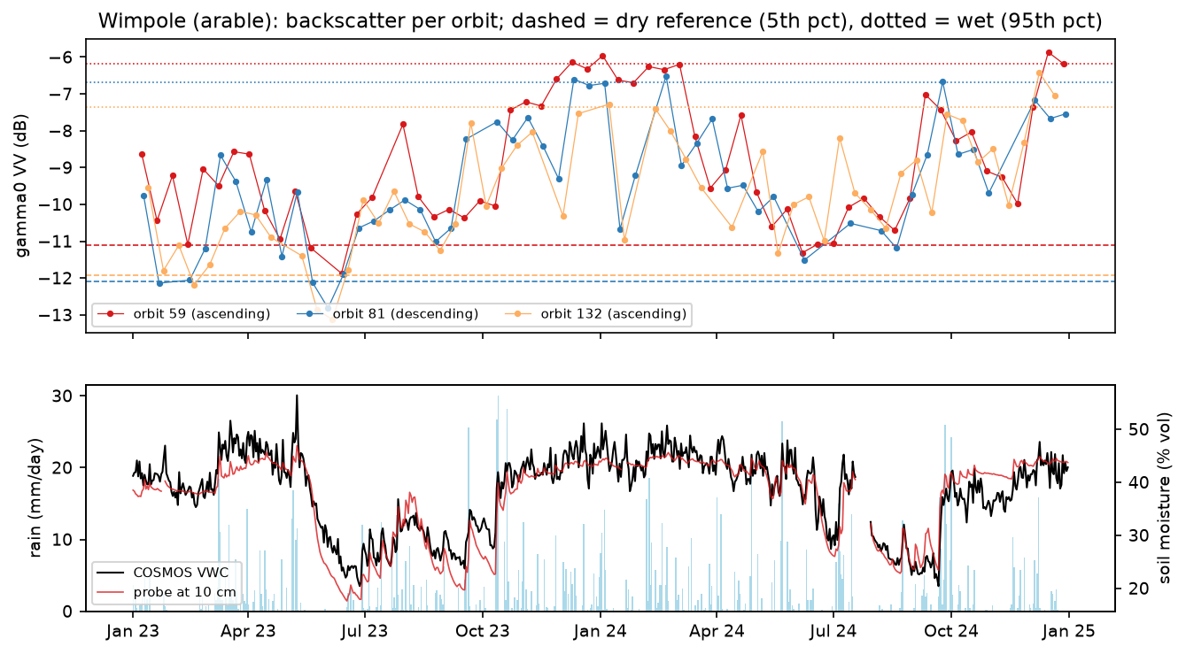
The radar tracks the broad seasonal cycle, but with large swings from one pass to the next. Some of those are real: the top few centimetres wet up within hours of rain and dry out within days, much faster than the soil at 10–30 cm. Others are crop growth, harvest and ploughing.

Step 4: how well does it agree with COSMOS-UK?

We match each Sentinel-1 date with the same day’s COSMOS value and compute Pearson’s r. To see what each modelling choice buys us, we also correlate the raw decibels and the pooled-orbit version, and we split the record into October–March (little vegetation) and April–September (crops and grass growing).

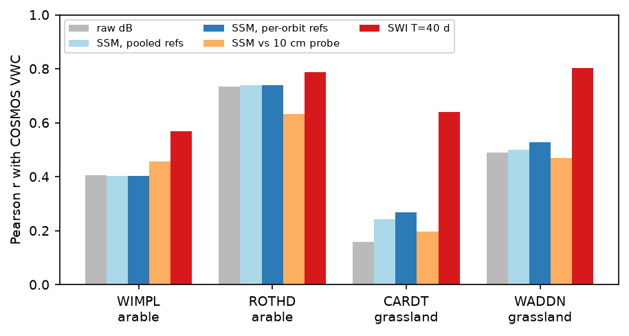
for s, df in s1.items():
    m = df.merge(insitu[s], left_on="date", right_index=True, how="inner").dropna(subset=["cosmos_vwc"])
    m["rain_3d"] = [insitu[s].precip.loc[d - pd.Timedelta(days=2):d].sum() for d in m.date]
    winter = m.date.dt.month.isin([10, 11, 12, 1, 2, 3])
    rows.append({"site": s, "cover": SITES[s][1], "n": len(m),
                 "r_cosmos": stats.pearsonr(m.ssm, m.cosmos_vwc)[0],
                 "r_pooled_orbits": stats.pearsonr(m.ssm_pooled, m.cosmos_vwc)[0],
                 "r_raw_dB": stats.pearsonr(m.vv_db, m.cosmos_vwc)[0],
                 "r_Oct-Mar": stats.pearsonr(m[winter].ssm, m[winter].cosmos_vwc)[0],
                 "r_Apr-Sep": stats.pearsonr(m[~winter].ssm, m[~winter].cosmos_vwc)[0]})

 site     cover   n  r_cosmos  r_tdt10cm  r_pooled_orbits  r_raw_dB  r_Oct-Mar  r_Apr-Sep  rmse_vwc_%
WIMPL    arable 163      0.40       0.46             0.40      0.41       0.45       0.11        8.45
ROTHD    arable 104      0.74       0.63             0.74      0.74       0.49       0.71        5.22
CARDT grassland 154      0.27       0.20             0.24      0.16       0.41       0.06        8.79
WADDN grassland 216      0.53       0.47             0.50      0.49       0.42       0.28        8.41
r_pooled_orbits: one dry/wet reference for all orbits (no incidence-angle handling)
rmse_vwc_%: relative SSM rescaled to the station's 5th-95th percentile VWC range

mean relative SSM (%) and COSMOS VWC (%) by rain in the previous 3 days:
 site  n_rain>=10mm_3d  ssm_after_rain  n_no_rain_3d  ssm_no_rain  cosmos_after_rain  cosmos_no_rain
WIMPL               32            73.8            43         25.0               41.3            34.5
ROTHD               23            73.7            20         33.4               36.8            31.4
CARDT               26            65.6            17         27.9               28.4            23.8
WADDN               45            71.8            49         36.3               44.1            36.8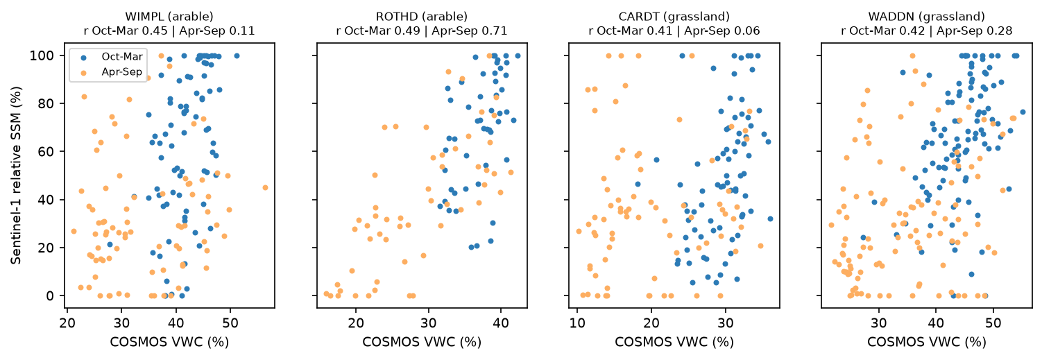

What the numbers say:

• It works, moderately. Same-day r ranged from 0.27 (Cardington) to 0.74 (Rothamsted). That is typical of published C-band validations at single sites, where r = 0.4–0.7 is common.
• The rain response is clear everywhere. After 10 mm or more of rain in three days, relative soil moisture averaged 66–74 %. After three dry days, it averaged 25–36 %. The radar responds to rain much more strongly than COSMOS does, because it sees only the wetted surface.
• Vegetation breaks it in summer. At Wimpole, Cardington and Waddesdon, r fell to 0.06–0.28 in April–September. Rothamsted is the exception (0.71). Its deep summer drying (down to 15 % by volume) dominates the range there, and that drying is large enough to show through the crop.
• Per-orbit references help only a little here. Pooling the orbits changed r by at most 0.03. The angle effect (under 1 dB) is small next to a 5 dB arable range. On grassland, with a 2 dB range, it matters more (0.24 vs 0.27 at Cardington, 0.50 vs 0.53 at Waddesdon). Over hilly ground or with orbits at very different angles, it matters much more.

Step 5: from the surface to the root zone with a soil water index

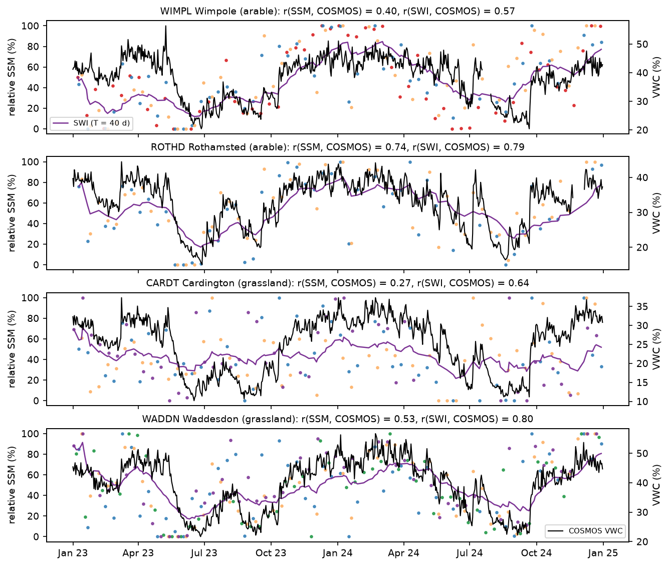
COSMOS integrates the top 10–30 cm, while C-band sees the top 1–5 cm. TU Wien bridges the gap with the soil water index, a recursive exponential filter with a characteristic time T in days. It smooths the surface series and lags it, roughly as infiltration does.

def soil_water_index(times: pd.Series, ssm: pd.Series, t_days: float) -> np.ndarray:
    """Recursive exponential filter (Albergel et al. 2008): a smoothed, lagged, deeper-layer proxy."""
    t = (times - times.iloc[0]).dt.total_seconds().to_numpy() / 86400
    swi, gain = np.empty(len(ssm)), 1.0
    swi[0] = ssm.iloc[0]
    for n in range(1, len(ssm)):
        gain = gain / (gain + np.exp(-(t[n] - t[n - 1]) / t_days))
        swi[n] = swi[n - 1] + gain * (ssm.iloc[n] - swi[n - 1])
    return swi

 site     cover  r_SSM  r_SWI_T1  r_SWI_T5  r_SWI_T10  r_SWI_T20  r_SWI_T40  r_SWI_T60
WIMPL    arable   0.40      0.41      0.47       0.51       0.55       0.57       0.55
ROTHD    arable   0.74      0.74      0.80       0.84       0.84       0.79       0.73
CARDT grassland   0.27      0.28      0.38       0.46       0.55       0.64       0.65
WADDN grassland   0.53      0.54      0.66       0.72       0.78       0.80       0.77
best characteristic time length on average: T = 40 days

The soil water index lifts the agreement at every site, to r = 0.57–0.80 at T = 40 days. Rothamsted peaks earlier, at T = 10–20 days. Part of this gain is genuine, because it matches the depths. Part is just averaging away speckle and vegetation noise. Note that we chose T by looking at the in-situ data, so the best value is slightly optimistic.

Step 6: 100 m relative soil moisture maps

To make a map, we apply the same model to every pixel. We read 52 dates of orbit 81 around Wimpole, 12 × 12 km, straight onto a 100 m grid. GDAL’s average resampling in the WarpedVRT averages the 10 × 10 native pixels in linear units, which is a cheap multilook that removes most of the speckle. ESA WorldCover 2021 keeps only grassland and cropland, where the model is meant to work. The map straddles 0° longitude, so it needs two WorldCover tiles.

MAP_ORBIT, MAP_RES, MAP_HALF = 81, 100, 6000
map_tr = from_origin(round(cx, -2) - MAP_HALF, round(cy, -2) + MAP_HALF, MAP_RES, MAP_RES)
items = list(catalog.search(collections=["sentinel-1-rtc"], bbox=(lon0 - 0.1, lat0 - 0.06, lon0 + 0.1, lat0 + 0.06),
                            datetime=f"{START}/{END}", query={"sat:relative_orbit": {"eq": MAP_ORBIT}}).items())
with ThreadPoolExecutor(8) as ex:   # GDAL "average" resampling = 10 x 10 multilook in linear units
    chips = list(ex.map(lambda i: read_mean(i.assets["vv"].href, map_tr, MW, MW, Resampling.average), items))
# ... merge slices by date into `cube` (dates, y, x), in dB ...

dry_ref, wet_ref = np.nanpercentile(cube, LO, axis=0), np.nanpercentile(cube, HI, axis=0)
ssm_cube = np.clip(100 * (cube - dry_ref) / (wet_ref - dry_ref), 0, 100)
soil = np.isin(wc, [30, 40])            # WorldCover grassland and cropland

We pick three dates using the Wimpole station: the driest day after five rain-free days, the wettest October–March date, and the wettest April–June date, when crops were growing, among the 52 orbit 81 dates.

52 dates on a 120 x 120 grid of 100 m (100.0% valid); grassland+cropland = 87% of pixels
median sensitivity (wet - dry) on cropland 7.68 dB, grassland 3.16 dB, tree cover 2.45 dB, built-up 2.64 dB
               case        date  COSMOS_vwc_%  rain_prev_5d_mm  median_SSM_cropland_%  median_SSM_grassland_%
                dry 31 Aug 2024          22.5              0.0                   38.2                    29.3
       wet (winter) 04 Jan 2024          47.8             38.1                   95.9                    83.9
wet (crops growing) 09 May 2023          56.4             51.3                   27.4                    68.6
area-median SSM (grass+crop) vs Wimpole COSMOS over 52 dates: r = 0.37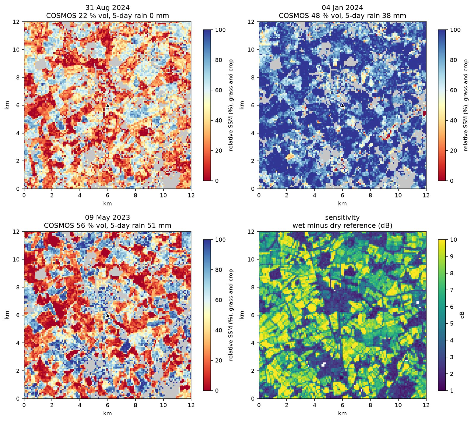

The winter map behaves as expected: after 38 mm of rain, nearly every field is near its wet reference (median 96 % on cropland). The dry map is patchy, because fields differ in crop residue, tillage and stubble. The 9 May 2023 map is the warning. It was the wettest day of the two-year record (56 % by volume), but cropland had a median of only 27 %. In May, winter wheat and oilseed rape are tall, wet canopies that scatter and absorb the radar before it reaches the soil. The sensitivity map shows the other side of the same problem: arable fields have 7–10 dB of range, more than soil moisture alone can produce, because tillage and crop growth add to it.

Limitations and how to improve them

• Vegetation. The biggest error. The operational TU Wien algorithm models the seasonal vegetation effect from the incidence-angle slope. Simpler options are to mask the growing season on arable land, use the VH/VV ratio to flag dense canopy (see Sentinel-1 crop monitoring), or use a water cloud model with Sentinel-2 NDVI.
• Roughness and tillage. Ploughing can shift a field’s backscatter by several decibels in a day. A long record and percentile references dampen this, but a field that is ploughed every autumn will show “wet” ploughed soil.
• Incidence angle. We avoided normalisation by keeping a reference per orbit. Over hills, or to combine orbits into one reference, normalise to a common angle with a per-pixel slope. The RTC collection on the Planetary Computer has no incidence angle band, so you would need the GRD annotation files or a geometry model.
• Depth mismatch. C-band senses 1–5 cm; COSMOS 10–30 cm; the TDT probe a point at 10 cm. Low same-day r is partly a scale problem, not an error in the radar.
• Record length. Two years is short for the references. TU Wien uses the whole Sentinel-1 archive. If 2023–2024 never reached a truly dry or wet state at some pixel, its scale is stretched.
• Speckle. Footprint and 100 m averaging handle it here. For 10–20 m maps, filter first; see SAR speckle filtering in Python.

Frequently asked questions

Can Sentinel-1 measure soil moisture?

Yes, in the top few centimetres and in relative terms. Wet soil has a higher dielectric constant, so it returns more C-band backscatter. Change detection turns that into a 0–100 % index per pixel. Copernicus publishes an operational 1 km surface soil moisture product from Sentinel-1 based on the same TU Wien method. In this tutorial, the same-day correlation with field-scale in-situ sensors was 0.27–0.74, and 0.57–0.80 after filtering into a soil water index.

What is the change detection method for soil moisture?

It scales each backscatter value between a pixel’s own driest and wettest observed values: SSM = (σ⁰ − σ⁰dry) / (σ⁰wet − σ⁰dry). The references come from a long time series, often as low and high percentiles, and the operational version normalises backscatter to a 40° incidence angle first. Because each pixel is compared only with itself, constant effects of soil type and roughness cancel out.

Should I use VV or VH for soil moisture?

VV. Co-polarised backscatter responds more strongly to the soil surface. VH comes mostly from volume scattering in vegetation, so it is more useful as a vegetation indicator, for example to flag dates when the canopy is too dense for a reliable soil moisture estimate.

How deep does Sentinel-1 see into the soil?

C-band (5.6 cm wavelength) penetrates roughly 1–5 cm into moist soil, and a little deeper into very dry soil. That is why the radar reacts within hours to rain that deeper sensors barely notice. To estimate root-zone moisture, use a soil water index or assimilate the observations into a land surface model.

How does vegetation affect SAR soil moisture?

A crop or grass canopy both adds its own backscatter and attenuates the signal from the soil. When the canopy is dense, the radar sees the plants, not the soil. Here, agreement with in-situ soil moisture fell to r = 0.06–0.28 in the growing season at three of four sites, and growing crops made cropland look dry on the wettest day of the record.

Is there a free Sentinel-1 soil moisture product?

Yes. The Copernicus Land Monitoring Service publishes a 1 km Surface Soil Moisture product from Sentinel-1, and a fused soil water index, using the TU Wien change-detection method. For coarser, longer records, ESA CCI Soil Moisture combines many satellites, and reanalyses such as ERA5-Land model soil moisture in layers. Building it yourself, as here, gives you 100 m or finer resolution and full control of the masking.

Next steps

• Learn the radar basics, decibels and the Lee filter in Sentinel-1 SAR flood mapping in Python.
• Flag dense crop canopies with VH and the VH/VV ratio in Sentinel-1 crop monitoring in Python.
• Filter speckle for 10–20 m soil moisture maps with SAR speckle filtering in Python.
• Compare with modelled soil moisture layers from ERA5-Land, opened with xarray as in ERA5 in Python with xarray.
• Use the same “compare with your own history” idea for disasters in earthquake damage mapping with Sentinel-1.
• Run the same model on more COSMOS-UK stations: the API lists over 50, from upland peat to chalk downland.

Data and licences

• Sentinel-1 RTC: contains modified Copernicus Sentinel data 2023–2024, processed by ESA; radiometric terrain correction by Catalyst/Microsoft. Licensed CC BY 4.0. Accessed from the Microsoft Planetary Computer on 23 October 2026.
• COSMOS-UK: daily soil moisture, TDT probe and rainfall data © UK Centre for Ecology & Hydrology, available under the Open Government Licence v3.0. Accessed through the COSMOS-UK API on 23 October 2026.
• ESA WorldCover 2021: © ESA WorldCover project 2021 / contains modified Copernicus Sentinel data (2021) processed by the ESA WorldCover consortium, licensed CC BY 4.0. Accessed from the Microsoft Planetary Computer.
• Code: soil_moisture.py, tested with Python 3.12.0, pystac-client 0.9.1, planetary-computer 1.0.0, rasterio 1.5.2, numpy 2.5.4, scipy 1.18.1 and pandas 3.1.0.