Earthquake damage mapping with Sentinel-1 in Python: log ratio and z-scores in Antakya

Short answer: to map earthquake damage with Sentinel-1 in Python, compare the first post-event image with the images before the event, on the same orbit.

• The simplest test is the log ratio, 10·log10(post / pre) in decibels.
• A more robust test is a z-score against a pre-event stack: (post − mean_pre) / sd_pre for each pixel.
• Mask to built-up land, count the share of pixels with |z| > 2 in grid cells, and threshold that share, for example with Otsu’s method.

For Antakya after the February 2023 earthquakes, this ranked 200 m cells with destroyed buildings with an AUC of 0.84. Read it as a neighbourhood-level damage proxy: 10 m amplitude does not resolve individual buildings.

On 6 February 2023, two earthquakes of magnitude 7.8 and 7.5 struck south-east Türkiye and north-west Syria. More than 50,000 people died. Antakya, the old city of Antioch in Hatay province, was among the worst hit: whole blocks of its old town collapsed. Cloud and smoke did not matter to Sentinel-1, which imaged the city on 9, 10 and 15 February from three different orbits.

In this tutorial, we turn those images into a damage map and, unusually for a tutorial, test it against an independent reference: the 730 destroyed buildings that Humanitarian OpenStreetMap Team (HOT) volunteers mapped in our study area.

You will learn how to:

1. stream a pre-event Sentinel-1 stack and the first post-event image for three orbits;
2. download a reference of destroyed buildings from the Humanitarian Data Exchange;
3. compute the log ratio and a z-score against the pre-event stack, with a no-event control;
4. aggregate pixel changes into a 200 m damage index on built-up land;
5. measure how well the index ranks damaged cells with ROC AUC;
6. pick a threshold without the reference, then build a confusion table and kappa.

All outputs below are real results from damage_mapping.py, run on 23 October 2026 with Python 3.12, pystac-client 0.9.1, rasterio 1.5.2 and geopandas 1.2.0. A full run takes under a minute on a home broadband connection.

How does SAR detect earthquake damage?

A standing building is a strong radar reflector. The wall and the ground form a double-bounce corner that sends the pulse straight back to the satellite, so cities are bright in SAR images. When a building collapses, the corner is destroyed and the rubble scatters the pulse in all directions. Backscatter usually drops. But it can also rise, for example when debris forms new corners, or when a neighbouring building that was in shadow becomes visible. So we look for change in either direction.

There are two families of methods:

• Amplitude (intensity) change, used here. It works with the analysis-ready backscatter that the Planetary Computer serves as Cloud Optimised GeoTIFFs.
• Coherence change, used by the damage proxy maps of NASA JPL/ARIA and the Earth Observatory of Singapore. Interferometric coherence measures whether the fine structure of each pixel stayed the same between two passes. It is more sensitive to damage, but it needs complex single look complex (SLC) data and interferometric processing. See InSAR ground deformation in Python for what that involves.

Step 1: a pre-event stack and the first post-event image

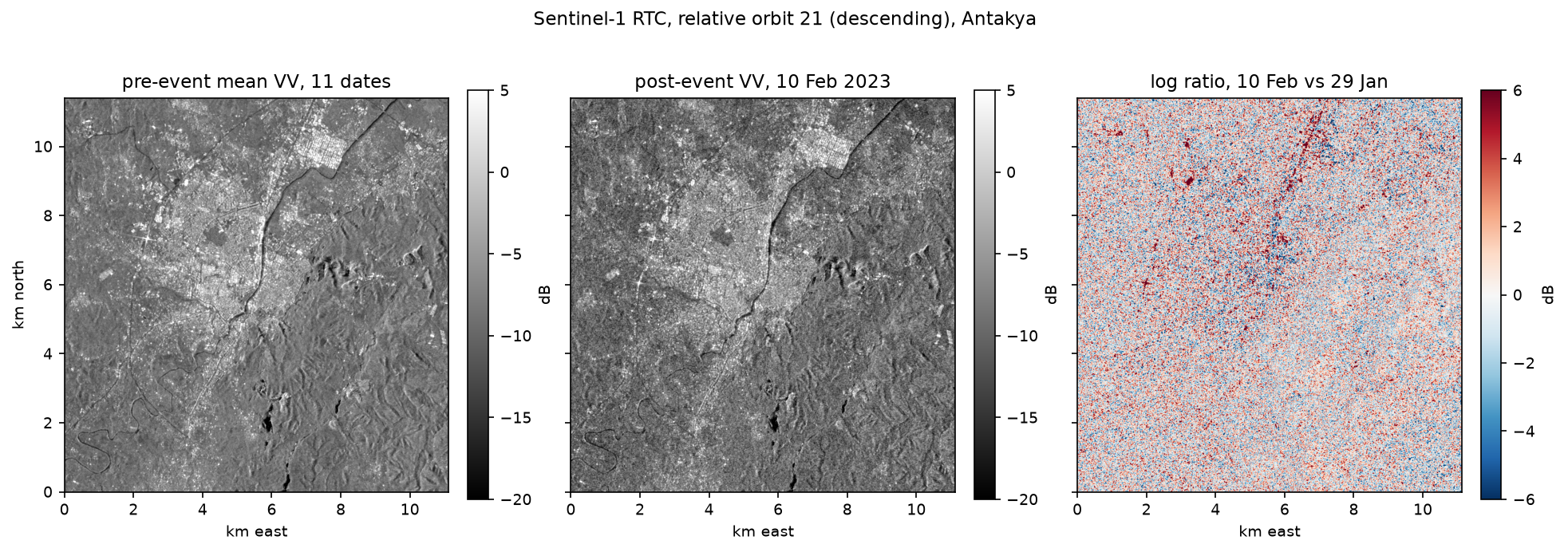
We define a 10 × 11 km box over Antakya and read every Sentinel-1 RTC scene from 1 October 2022 to 19 February 2023, for the three relative orbits that cover the city. Each scene is warped onto one 10 m UTM grid with a WarpedVRT. A pass can be split into two slices that both cover the town, so we merge them by acquisition time.

BBOX = (36.10, 36.15, 36.22, 36.25)        # lon/lat: Antakya (Hatay), Turkey
EVENT = pd.Timestamp("2023-02-06 01:17", tz="UTC")
ORBITS = {14: "ascending", 21: "descending", 94: "descending"}
CRS = "EPSG:32637"                          # UTM 37N
b = [round(v, -1) for v in transform_bounds(4326, CRS, *BBOX)]
TR = from_origin(b[0], b[3], 10, 10)
W, H = int((b[2] - b[0]) / 10), int((b[3] - b[1]) / 10)
catalog = pystac_client.Client.open("https://planetarycomputer.microsoft.com/api/stac/v1",
                                    modifier=planetary_computer.sign_inplace)


def read_band(item, band: str) -> np.ndarray:
    """Warp one RTC asset onto the common grid; 0 is nodata in the COGs."""
    with rasterio.open(item.assets[band].href) as src, \
            WarpedVRT(src, crs=CRS, transform=TR, width=W, height=H, nodata=0,
                      resampling=Resampling.bilinear) as vrt:
        a = vrt.read(1).astype("float32")
    a[a <= 0] = np.nan
    return a


def load_orbit(orbit: int) -> dict:
    items = list(catalog.search(collections=["sentinel-1-rtc"], bbox=BBOX, datetime="2022-10-01/2023-02-19",
                                query={"sat:relative_orbit": {"eq": orbit}}).items())
    jobs = [(i, band) for i in items for band in ("vv", "vh")]
    with ThreadPoolExecutor(8) as ex:
        arrays = list(ex.map(lambda j: read_band(*j), jobs))
    by_date = defaultdict(lambda: defaultdict(list))  # several slices can cover the town on one pass
    for (item, band), a in zip(jobs, arrays):
        by_date[item.datetime.strftime("%Y-%m-%dT%H:%M")][band].append(a)
    dates = sorted(by_date)
    return {"dates": pd.to_datetime(dates).tz_localize("UTC"),
            **{band: np.stack([np.nanmax(np.stack(by_date[d][band]), 0) for d in dates]) for band in ("vv", "vh")}}


s1 = {orbit: load_orbit(orbit) for orbit in ORBITS}

grid: 1112 x 1141 pixels of 10 m in EPSG:32637
 orbit       pass  pre_scenes   first_pre    last_pre  post_scenes  first_post  valid_%
    14  ascending          10 12 Oct 2022 28 Jan 2023            1 09 Feb 2023    100.0
    21 descending          11 01 Oct 2022 29 Jan 2023            1 10 Feb 2023    100.0
    94 descending          11 06 Oct 2022 03 Feb 2023            1 15 Feb 2023    100.0
read in 34.4 s

Each orbit has 10–11 pre-event images, one every 12 days (Sentinel-1B had failed in December 2021, so only Sentinel-1A was imaging), and one post-event image 3–9 days after the earthquakes. Always compare images from the same orbit: different orbits see buildings from different directions and angles, so their backscatter differs far more than any damage signal.

Step 2: a reference of destroyed buildings

To test a damage map you need an independent reference. The obvious candidates were not usable:

• Copernicus EMS rapid mapping (activation EMSR648) graded buildings in Antakya, but its products for that activation could not be downloaded at the time of writing: the current EMS API lists only activations from EMSR656 onwards, and the old download links return 404.
• UNOSAT published damage points for the event, but the openly downloadable set covers Syrian towns, not Antakya.

So we use the HOT destroyed-buildings export on the Humanitarian Data Exchange. After the earthquakes, OpenStreetMap volunteers tagged buildings that had collapsed, tracing them from very high resolution imagery, including the Copernicus EMS products. The export is open under the ODbL. We find the current GeoPackage link through the HDX API, so the script keeps working if the file is refreshed.

pkg = requests.get("https://data.humdata.org/api/3/action/package_show",
                   params={"id": "hotosm_tur_destroyed_buildings"}, timeout=60).json()["result"]
url = next(r["url"] for r in pkg["resources"] if r["url"].endswith(".zip") and "gpkg" in r["url"])
with zipfile.ZipFile(io.BytesIO(requests.get(url, timeout=300).content)) as zf:
    name = next(n for n in zf.namelist() if n.endswith(".gpkg"))
    REF.write_bytes(zf.read(name))
ref = gpd.read_file(REF)
print(f"{len(ref)} destroyed-building polygons in Turkey | sources: {ref['source'].value_counts().to_dict()}")
ref = ref.to_crs(CRS)
ref["geometry"] = ref.geometry.centroid
x0, y0 = TR.c, TR.f
ref = ref[(ref.geometry.x > x0) & (ref.geometry.x < x0 + W * 10) & (ref.geometry.y < y0) & (ref.geometry.y > y0 - H * 10)]

3239 destroyed-building polygons in Turkey | sources: {'cscrs': 1542, 'CopernicusEMS': 739, 'microsoft/BuildingFootprints': 115, 'cscrc': 107, 'OpenAerialMap': 31, 'mapillary': 5, 'HGM': 3, 'SkySat': 3, ...}
730 of them inside the Antakya study area

We also need a built-up mask, because damage only happens where there are buildings, and fields and forests change for other reasons. ESA WorldCover 2021 (class 50) gives one: built-up land covers 25.3 % of the box, or 32.1 km².

Step 3: log ratio and z-score against the pre-event stack

The log ratio compares the post-event image with one pre-event image. It is the textbook SAR change detector, but it treats every pixel the same, whether its backscatter normally varies by 0.5 dB or by 4 dB. The z-score divides the change by the pixel’s own pre-event standard deviation, so a 3 dB drop at a stable building counts for more than a 3 dB drop at a pixel that is always noisy.

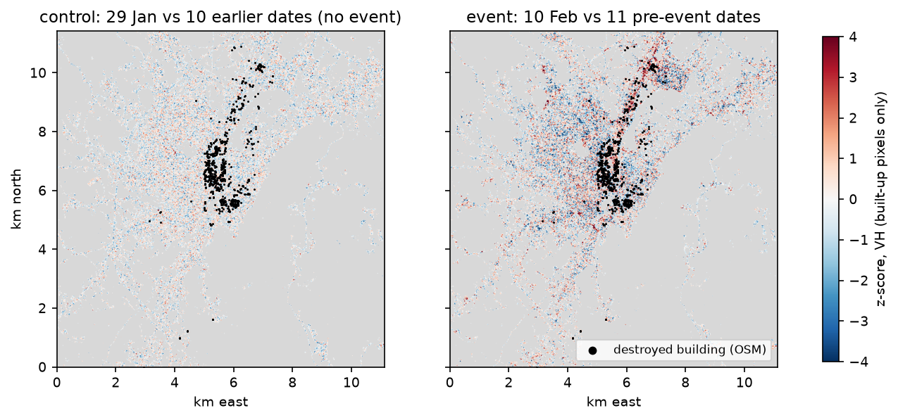
To see what “no earthquake” looks like, we also build a control: the last pre-event image scored against the earlier pre-event images. Any exceedance in the control is the false-alarm background from weather, construction and speckle.

for orbit, d in s1.items():
    pre = np.asarray(d["dates"] < EVENT)
    i_post = int(np.flatnonzero(~pre)[0])
    for pol in ("vv", "vh"):
        db = 10 * np.log10(d[pol])
        stack_db, post_db = db[pre], db[i_post]
        log_ratio = post_db - stack_db[-1]                 # dB difference = 10 log10(post / pre)
        mu, sd = stack_db.mean(0), stack_db.std(0, ddof=1)
        z = (post_db - mu) / sd
        z_pre = (stack_db[-1] - stack_db[:-1].mean(0)) / stack_db[:-1].std(0, ddof=1)  # a no-event control
        change[(orbit, pol)] = {"log_ratio": log_ratio, "z": z, "z_control": z_pre}

 orbit pol   post  built_sd_dB  |LR|>3dB_%  |z|>2_%  |z|>2_%_control
    14  VV 09 Feb         1.71        30.2     19.2              8.6
    14  VH 09 Feb         1.64        28.3     18.4              9.3
    21  VV 10 Feb         1.74        29.7     18.6              7.6
    21  VH 10 Feb         1.64        28.9     19.5              8.3
    94  VV 15 Feb         1.41        27.3     22.6              9.0
    94  VH 15 Feb         1.41        23.5     19.5              8.4

exceedance by WorldCover class (mean of the 6 orbit/polarisation pairs):
land cover  pixels  |z|>2 % event  |z|>2 % control
tree cover  499947           11.4              8.9
 grassland  192410           11.0              8.5
  cropland  117546           11.5              8.4
  built-up  321099           19.6              8.5

The typical built-up pixel varies by 1.4–1.7 dB from date to date, so a 3 dB log ratio threshold flags 24–30 % of built-up pixels: mostly speckle. The z-score is better behaved. In the control, about 8.5 % of pixels exceed |z| = 2 on every land cover class. After the earthquakes, that rose only a little on trees, grass and crops (to about 11 %), but more than doubled on built-up land (19.6 %). That contrast, specific to buildings, is the damage signal.

Step 4: aggregate to a 200 m damage index

Single 10 m pixels are too noisy to call damage. Instead, we count, in each 200 m cell, the share of built-up pixels with |z| > 2, and average that over the 6 orbit and polarisation pairs. We score only cells that are at least half built-up, and we label a cell as damaged in the reference if it contains at least one destroyed building.

def grid_stats(cell_px: int):
    h, w = H // cell_px, W // cell_px

    def agg(a):
        a = np.where(built, a, np.nan)[:h * cell_px, :w * cell_px].reshape(h, cell_px, w, cell_px)
        return np.nanmean(a, axis=(1, 3))

    built_frac = built[:h * cell_px, :w * cell_px].reshape(h, cell_px, w, cell_px).mean(axis=(1, 3))
    cols = ((ref.geometry.x - TR.c) / (10 * cell_px)).astype(int).to_numpy()
    rws = ((TR.f - ref.geometry.y) / (10 * cell_px)).astype(int).to_numpy()
    ok = (rws < h) & (cols < w)
    count = np.zeros((h, w))
    np.add.at(count, (rws[ok], cols[ok]), 1)
    z_index = np.mean([agg((np.abs(c["z"]) > 2).astype("float32")) for c in change.values()], axis=0)
    lr_index = np.mean([agg(np.abs(c["log_ratio"])) for c in change.values()], axis=0)
    ctrl_index = np.mean([agg((np.abs(c["z_control"]) > 2).astype("float32")) for c in change.values()], axis=0)
    per_combo = {k: agg((np.abs(c["z"]) > 2).astype("float32")) for k, c in change.items()}
    return built_frac, count, z_index, lr_index, ctrl_index, per_combo


CELL = 20                                       # 20 x 10 m = 200 m
built_frac, count, z_index, lr_index, ctrl_index, per_combo = grid_stats(CELL)
sel = built_frac >= 0.5                         # score only cells that are at least half built-up
label = count[sel] >= 1

732 cells of 200 m are >= 50 % built-up; 116 contain >= 1 destroyed building (698 of 730 reference buildings fall in scored cells)
damage index (mean share of built pixels with |z| > 2 over 6 orbit/polarisation pairs): median 0.200, 95th pct 0.330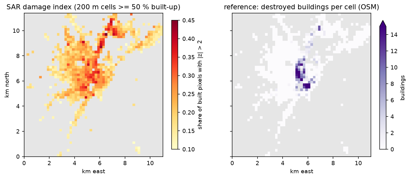

Step 5: does the index rank damaged cells first?

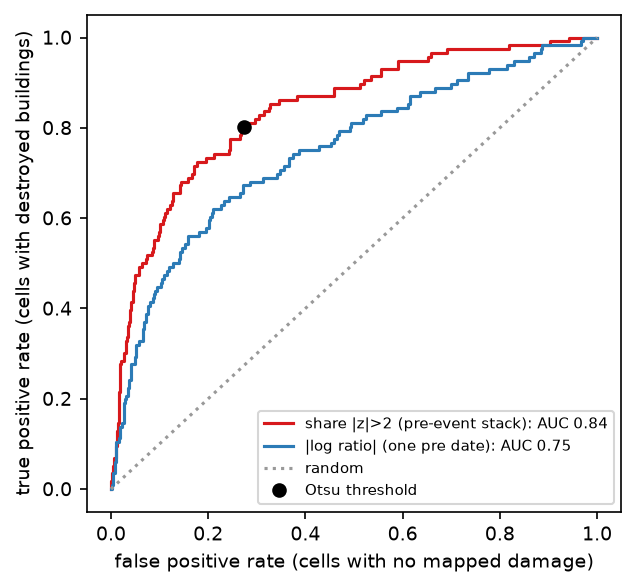
ROC AUC answers a simple question: if you pick one cell with mapped destruction and one without, how often does the damaged cell have the higher score? We compute it with the Mann-Whitney U statistic, so no threshold is needed yet.

def auc(score, label):
    """ROC AUC via the Mann-Whitney U statistic (probability a damaged cell outranks an undamaged one)."""
    r = stats.rankdata(score)
    n1, n0 = label.sum(), (~label).sum()
    return float((r[label].sum() - n1 * (n1 + 1) / 2) / (n1 * n0))

                   score   AUC
  |log ratio|, mean of 6 0.749
  share |z|>2, mean of 6 0.838
share |z|>2, orbit 14 VV 0.790
share |z|>2, orbit 14 VH 0.744
share |z|>2, orbit 21 VV 0.781
share |z|>2, orbit 21 VH 0.791
share |z|>2, orbit 94 VV 0.772
share |z|>2, orbit 94 VH 0.774
Spearman rho (damage index vs number of destroyed buildings per cell) = 0.433, p = 9.3e-35

sensitivity to cell size and reference threshold:
 cell_m  damaged_if_>=  cells  damaged  AUC_logratio  AUC_zindex
    100              1   3150      242         0.723       0.825
    100              3   3150       90         0.717       0.828
    200              1    732      116         0.749       0.838
    200              3    732       65         0.730       0.845
    400              1    175       51         0.757       0.858
    400              3    175       38         0.755       0.860

Three lessons:

1. The pre-event stack helps. The z-index (AUC 0.84) clearly beats the mean absolute log ratio (0.75).
2. More looks help. Any single orbit and polarisation reaches 0.74–0.79; averaging all six reaches 0.84. If you have only the first post-event pass, expect the lower figure.
3. Coarser cells score better (0.83 at 100 m, 0.86 at 400 m), because more pixels average out speckle. The trade-off is a coarser map.

Step 6: a threshold without the reference, and the agreement table

In a real emergency there is no reference, so the threshold has to come from the data. We compare four rules: the 99th percentile of the no-event control index, Otsu’s method on the event index, and the event mean plus one or two standard deviations. Then we score each with precision, recall, F1, overall accuracy and Cohen’s kappa.

def otsu(values: np.ndarray, bins: int = 64) -> float:
    """Otsu's threshold: maximise the between-class variance of a histogram."""
    hist, edges = np.histogram(values, bins)
    centres = (edges[:-1] + edges[1:]) / 2
    best, best_var = centres[0], -1.0
    for k in range(1, bins):
        w0, w1 = hist[:k].sum(), hist[k:].sum()
        if w0 == 0 or w1 == 0:
            continue
        m0, m1 = (hist[:k] * centres[:k]).sum() / w0, (hist[k:] * centres[k:]).sum() / w1
        if w0 * w1 * (m0 - m1) ** 2 > best_var:
            best, best_var = centres[k], w0 * w1 * (m0 - m1) ** 2
    return float(best)


v = z_index[sel]
thresholds = {"control 99th pct": float(np.percentile(ctrl_index[sel], 99)),
              "Otsu on event index": otsu(v),
              "event mean + 1 sd": float(v.mean() + v.std()),
              "event mean + 2 sd": float(v.mean() + 2 * v.std())}
rows = [{"rule": k, "threshold": round(t, 3), **agreement(v > t, label)} for k, t in thresholds.items()]

               rule  threshold  flagged  precision  recall    f1  overall_accuracy  kappa
   control 99th pct      0.120      712      0.163   1.000 0.280             0.186  0.011
Otsu on event index      0.226      261      0.356   0.802 0.493             0.739  0.351
  event mean + 1 sd      0.271      111      0.541   0.517 0.529             0.854  0.442
  event mean + 2 sd      0.331       34      0.706   0.207 0.320             0.861  0.267

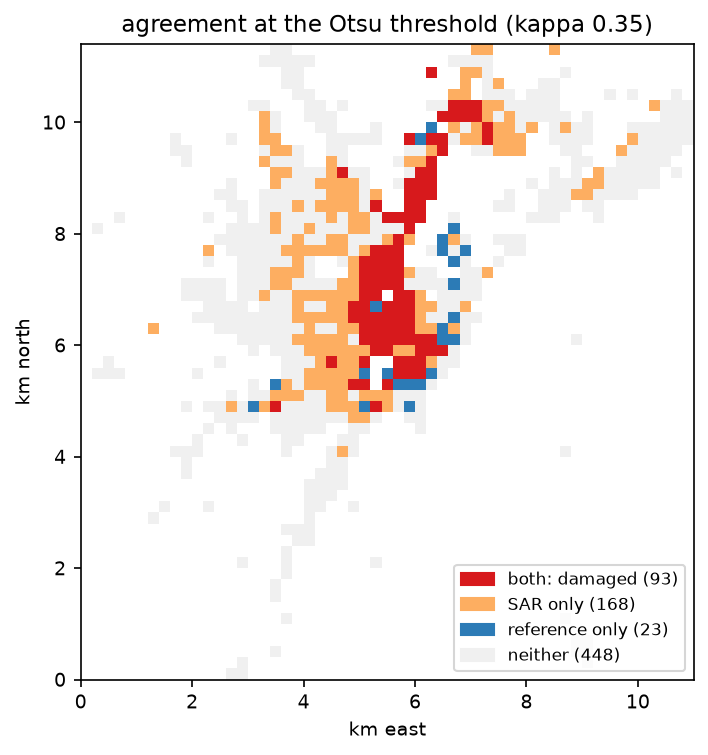
confusion table at the Otsu threshold (0.226), 200 m built-up cells:
                           SAR: damaged  SAR: not flagged  total
reference: >= 1 destroyed            93                23    116
reference: none mapped              168               448    616
total                               261               471    732
odds ratio 10.8; Fisher exact p = 6.9e-27

The control threshold is a useful warning. A cell that would be unusual in a normal 12-day interval is everywhere after the earthquake: 712 of 732 cells (97 %) exceed it. The change after the event is city-wide, so “anything unusual” is not a useful definition of damage.

Otsu gives a sensible operating point. It flags 261 cells, catches 93 of the 116 cells with mapped destroyed buildings (recall 0.80), and a flagged cell is 10.8 times more likely, in odds, to contain mapped destruction. Precision is only 0.36, but many of the 168 “SAR only” cells may well be damaged buildings that nobody mapped. A stricter rule (mean + 1 sd) gives the best kappa (0.44) at the cost of missing half the damaged cells. For a first triage map, recall usually matters more.

What can go wrong: weather and other false alarms

Before you trust a single post-event image, check how often normal dates look just as unusual. Here we score every pre-event date against the other pre-event dates, leaving the date out, and plot the share of built-up pixels with |z| > 2, separately for cells with three or more destroyed buildings and cells with none.

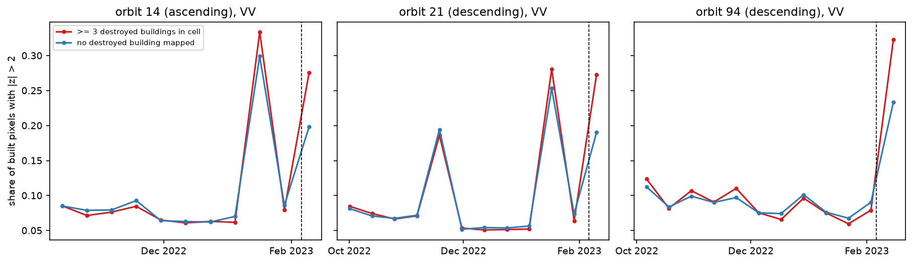
On 16 and 17 January, exceedance jumped to 0.25–0.33 with no earthquake: probably rain or wet snow changing the surfaces of the whole city. What distinguishes the earthquake is not the size of the change but the gap between damaged and undamaged cells. In practice:

• check the weather on the post-event date and use several post-event passes if you can;
• use a robust baseline (median and median absolute deviation) so that one wet date in the stack does not inflate the standard deviation;
• compare with a no-event control, as we did, before setting thresholds.

Limitations and how to improve them

• Resolution. At 10 m, with speckle, one Sentinel-1 pixel covers a whole small building. This method maps damaged neighbourhoods, not damaged buildings. For building-level assessment, use very high resolution optical or SAR imagery, as the Copernicus EMS and UNOSAT analysts do.
• Amplitude only. Coherence loss is the more sensitive damage indicator, but it needs SLC data and interferometric processing. The Earth Observatory of Singapore’s Remote Sensing Lab (EOS-RS) published coherence-based damage proxy maps for this event.
• It does not always work. We tried the same approach for Mandalay and Sagaing after the 28 March 2025 Myanmar earthquake, against UNOSAT damage points, and found no useful signal (AUC about 0.5). We did not establish why; plausible reasons include more scattered damage, smaller buildings and a different mix of partial and total collapse. Test your method against a reference before relying on it.
• Incomplete reference. The HOT export lists only destroyed buildings and is spatially uneven. A graded reference (destroyed, damaged, possibly damaged) such as Copernicus EMS gradings would allow a fairer test.
• Other changes. Rubble clearance, tent camps, displaced vehicles and weather all change backscatter. The first post-event image is the cleanest; later ones mix in the recovery.
• Thresholds. Otsu worked here because damage was widespread. Where damage is rare, the histogram is not bimodal and Otsu will pick an arbitrary split; use a control-based or fixed threshold instead.

Frequently asked questions

Can Sentinel-1 detect earthquake damage?

Yes, at the neighbourhood scale. Collapsed buildings lose the double-bounce reflection that makes cities bright in radar, and the rubble changes backscatter. In Antakya, a 200 m index of unusual change ranked cells with destroyed buildings above the rest with an AUC of 0.84. Sentinel-1 cannot reliably assess individual buildings at 10 m resolution, and it found no clear signal in a test in Myanmar in 2025.

What is log ratio change detection in SAR?

It is the difference between two co-registered SAR images in decibels: 10·log10(post / pre). The ratio is used instead of a difference because SAR speckle is multiplicative, so a ratio gives the same statistics in bright and dark areas. Large positive or negative values mean change. It is simple and fast, but with only one pre-event image it cannot tell real change from a pixel’s normal variability.

Is coherence or amplitude better for damage mapping?

Coherence is usually more sensitive, because even partial damage scrambles the fine phase structure of a pixel. But it needs single look complex (SLC) data, precise co-registration and interferometric processing, and it is affected by vegetation and long time gaps. Amplitude change works with analysis-ready backscatter, such as the Planetary Computer’s RTC, and is easier to run quickly. Many operational products combine both.

How soon after an earthquake can Sentinel-1 map damage?

It depends on when the satellite next passes. With Sentinel-1A alone in 2023, each orbit repeated every 12 days, and Antakya was imaged 3, 4 and 9 days after the earthquakes on three orbits. With Sentinel-1C in orbit since December 2024, revisits are more frequent again. Processing the data with the script in this tutorial takes about a minute.

Why use a z-score instead of a simple difference?

Because pixels vary differently. A building that is stable within 0.5 dB and drops by 3 dB has changed far more than a noisy pixel that swings by 3 dB every 12 days. Dividing by each pixel’s pre-event standard deviation puts every pixel on the same scale. Here that lifted the ranking performance from an AUC of 0.75 for the log ratio to 0.84.

Where can I get reference damage data?

Copernicus EMS rapid mapping, UNOSAT and the Humanitarian Data Exchange publish damage assessments for major disasters, often as building points with damage grades. Availability varies: for this event, the EMS gradings for Antakya could no longer be downloaded, so we used the HOT/OpenStreetMap destroyed-buildings export. Read the methods note of any reference, because coverage is often incomplete.

Next steps

• Learn the radar basics, decibels and speckle filtering in Sentinel-1 SAR flood mapping in Python.
• Improve single-pixel change maps with SAR speckle filtering in Python.
• Measure ground movement from the same earthquake with interferometry: see InSAR ground deformation in Python.
• Map buildings themselves, as a better mask than WorldCover, in building footprints from LiDAR in Python.
• Apply the same “compare with your own history” idea to farmland in Sentinel-1 soil moisture in Python.

Data and licences

• Sentinel-1 RTC: contains modified Copernicus Sentinel data 2022–2023, processed by ESA; radiometric terrain correction by Catalyst/Microsoft. Licensed CC BY 4.0. Accessed from the Microsoft Planetary Computer on 23 October 2026.
• HOT destroyed buildings (Türkiye): © OpenStreetMap contributors, available under the Open Database Licence (ODbL). Exported by the Humanitarian OpenStreetMap Team and accessed from the Humanitarian Data Exchange on 23 October 2026.
• ESA WorldCover 2021: © ESA WorldCover project 2021 / contains modified Copernicus Sentinel data (2021) processed by the ESA WorldCover consortium, licensed CC BY 4.0. Accessed from the Microsoft Planetary Computer.
• Code: damage_mapping.py, tested with Python 3.12.0, pystac-client 0.9.1, planetary-computer 1.0.0, rasterio 1.5.2, geopandas 1.2.0, numpy 2.5.4, scipy 1.18.1 and pandas 3.1.0.