Multi-colour 3D-printed terrain with Python: one STL per colour for AMS and MMU printers
Split a 3D-printed model of Yr Wyddfa (Snowdon) into four watertight colour parts (water, woodland, open ground and high ground) from Copernicus GLO-30 and ESA WorldCover, remove specks too small to print, and write STLs and a 3MF for a Bambu Lab AMS or Prusa MMU.
- Level
- Advanced
- Tested with
- Python 3.12
- Source code
- Download scripts
Key takeaways
- A multi-colour terrain print is several watertight solids that share faces exactly. Cut them from one terrain solid with mesh booleans, then prove the volumes add up to the whole and no two parts overlap.
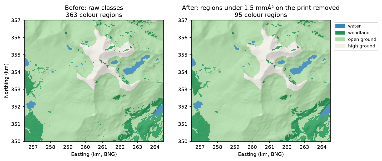
- Before cutting, sieve the colour map so that no region is smaller than you can print. Here that removed 268 of 363 regions while changing only 0.55% of cells.
- Thin colour caps over a single-colour body used 4.85 cm³ of accent filament instead of 59.18 cm³ for full-depth colour columns, but colour swaps were still needed on 144 of 159 layers.
- If your colours are only elevation bands, you do not need a multi-material unit: one filament change at the right z height does the job. The script prints that height for you.
Before you start
- Python 3.10+ with numpy, rasterio, scipy, shapely, manifold3d, pyvista and matplotlib
- Part 1 of this series, From DEM to 3D-printable STL, or familiarity with building a closed mesh from a height grid
- An internet connection (both rasters are streamed from public cloud-optimised GeoTIFFs)
- Optional: a multi-material printer (Bambu Lab AMS, Prusa MMU or similar) or a single-extruder printer with a pause or filament-change command
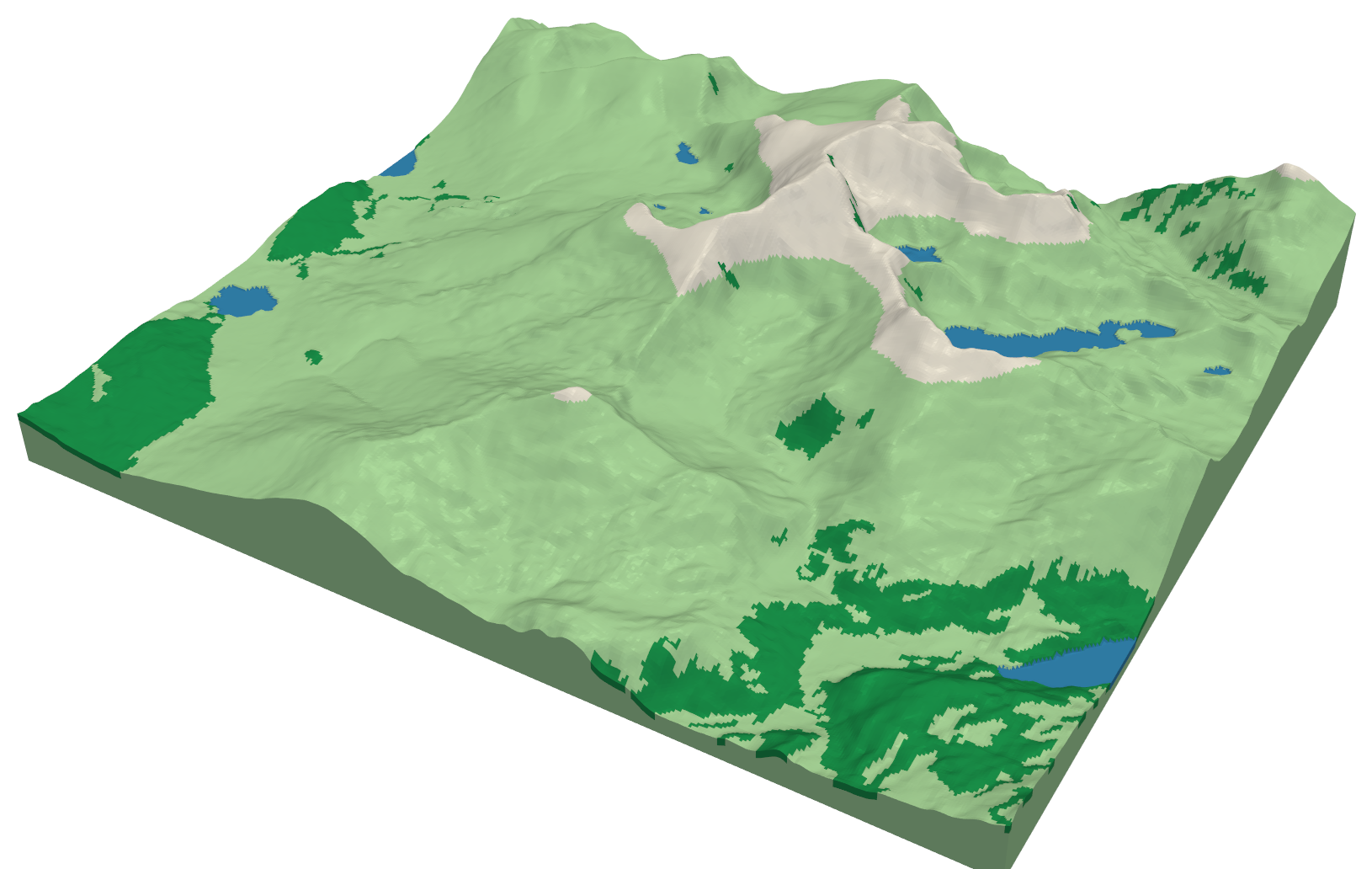
To print terrain in several colours, give the slicer one watertight solid per colour. The solids must fill the model between them with no gaps or overlaps. This tutorial builds that set of parts in Python for an 8 × 7 km model of Yr Wyddfa (Snowdon). There are four colours: lakes, woodland, open ground and high ground above 700 m. It also shows how to check that the parts really fit together before you load four spools.
Part 1 of this series, From DEM to 3D-printable STL, built one terrain solid with NumPy. Here we start from the same kind of solid and cut it into parts with manifold3d, a fast, exact mesh boolean library. The steps are:
- stream a Copernicus GLO-30 DEM and ESA WorldCover land cover onto one 20 m British National Grid;
- classify the map into four colours and remove regions too small to print;
- build the terrain solid, with lakes lowered slightly below their shores;
- cut one watertight part per colour, and compare full-depth colour with thin colour caps;
- write four STLs and a 3MF, then prove that the parts partition the model exactly.
The full script is multi_colour_terrain.py.
Step 1: terrain and land cover on one grid
Every colour boundary will become a vertical cut through the model, so the land cover and the heights must line up cell for cell. The simplest way to ensure that is to define the target grid once and have rasterio reproject both rasters straight into it:
AOI = (256_500, 350_000, 264_500, 357_000)      # 8 x 7 km around Yr Wyddfa, British National GridRES = 20.0X0, Y0, X1, Y1 = AOIDST = from_origin(X0, Y1, RES, RES)ROWS, COLS = int((Y1 - Y0) / RES), int((X1 - X0) / RES)
dem = np.full((ROWS, COLS), np.nan, dtype="float32")wc = np.zeros((ROWS, COLS), dtype="uint8")with rasterio.open(DEM_URL) as src:    reproject(rasterio.band(src, 1), dem, dst_transform=DST, dst_crs="EPSG:27700",              resampling=Resampling.bilinear, dst_nodata=np.nan)with rasterio.open(WC_URL) as src:    reproject(rasterio.band(src, 1), wc, dst_transform=DST, dst_crs="EPSG:27700",              resampling=Resampling.mode)
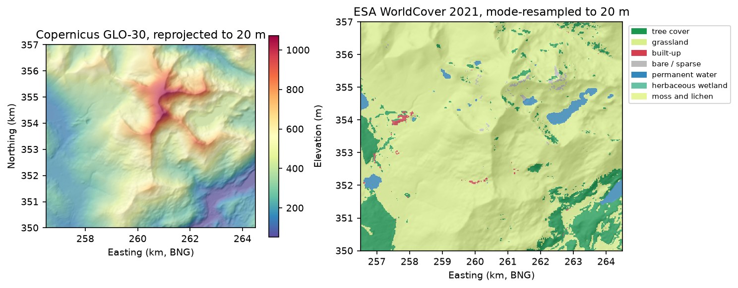
Heights use bilinear resampling. Land-cover classes are categories, not numbers, so they use mode: each 20 m cell takes the most common 10 m class beneath it. Averaging class codes would invent classes that do not exist.
=== Step 1: DEM and land cover on one 20 m grid ===grid 400 x 350 cells of 20 m | read and reprojected in 1.5 sDEM: 53.6 - 1072.6 m, NaNs 0WorldCover classes: tree cover 10.5%, grassland 86.7%, built-up 0.3%, bare / sparse 0.4%, permanent water 2.1%, herbaceous wetland 0.0%, moss and lichen 0.0%The highest cell is 1,072.6 m. The summit’s surveyed height is 1,085 m, but a 30 m surface model resampled to 20 m smooths a narrow peak. At 1:53,200 that difference is less than a quarter of a millimetre on the print.
Step 2: four printable colours, without the specks
A printer with an AMS or MMU can usually hold four filaments, so we reduce the map to four classes. Water and woodland come from WorldCover; everything else is split at 700 m into open ground and high ground:
lab = np.where(dem >= HIGH_M, 3, 2).astype("uint8") # 3 high ground, 2 open groundlab[wc == 10] = 1 # tree cover -> woodlandlab[wc == 80] = 0 # permanent waterThe raw map is full of one- and two-cell specks. Each would become a tiny island of colour, a few tenths of a millimetre across, that the printer cannot lay down cleanly and that adds needless colour swaps. The fix is a sieve: merge every region smaller than a threshold into its largest neighbour. We set the threshold in millimetres on the print, then convert it to cells, so the clean-up follows the print size rather than the data resolution:
scale = MODEL_LONG_MM / ((max(ROWS, COLS) - 1) * RES) # mm per metrecell_mm = RES * scalemin_px = int(np.ceil(MIN_REGION_MM2 / cell_mm ** 2)) # 1.5 mm2 -> cellslab = features.sieve(lab, size=min_px, connectivity=4)=== Step 2: classify into four colours and remove unprintable specks ===cell on the print 0.376 mm -> minimum region 1.5 mm2 = 11 cellswater regions 17 -> 11 | area 2.1% -> 2.1%woodland regions 273 -> 65 | area 10.5% -> 10.2%open ground regions 67 -> 16 | area 79.1% -> 79.5%high ground regions 6 -> 3 | area 8.3% -> 8.3%cells changed by the sieve: 772 (0.55%)The sieve removed 268 of 363 regions but changed only 772 cells. Most of the deleted regions were tiny, so the map looks almost the same and prints far better.
Step 3: the terrain solid
The terrain is a closed heightfield solid built exactly as in Part 1: a surface, a base with reversed winding and side walls. The code is in the heightfield_solid function in the script. Two changes help the colours. We use 1.5x exaggeration rather than 2x, because Snowdon is steep. And we lower the lake cells by 0.4 mm, so each lake reads as a flat, slightly recessed surface rather than a painted patch on the hillside:
Z = BASE_MM + (dem - dem.min()) * scale * Z_EXAGGERATIONZ[lab == 0] -= WATER_DROP_MMterrain = to_manifold(*heightfield_solid(Z, cell_mm))=== Step 3: terrain solid ===horizontal scale 1:53,200 | model 150.0 x 131.2 x 31.7 mmlakes lowered by 0.4 mm at 2,920 verticessingle-extruder alternative: change filament at z = 21.22 mm for ground above 700 mto_manifold hands the NumPy vertices and triangles to manifold3d. Manifold refuses meshes that are not closed and consistently wound, so it is a second check on the heightfield.
Step 4: one watertight part per colour
Each colour region becomes a prism: its outline from rasterio.features.shapes, extruded taller than the model. Intersect a prism with the terrain and you get that colour’s part. The outline must be in model millimetres, with pixel edges half a cell either side of the mesh vertices:
px_to_mm = rasterio.Affine(cell_mm, 0, -cell_mm / 2, 0, -cell_mm, (ROWS - 0.5) * cell_mm)
def class_prism(k):    contours = []    for geom, _ in features.shapes(lab, mask=lab == k, transform=px_to_mm, connectivity=4):        poly = orient(shape(geom), 1.0)              # outer rings anticlockwise, holes clockwise        contours += [np.array(poly.exterior.coords)[:-1]] + [np.array(h.coords)[:-1] for h in poly.interiors]    return mf.Manifold.extrude(mf.CrossSection(contours), Z.max() + 10).translate((0, 0, -5))
That leaves one design choice: how deep should a colour go?
- Design A, full-depth colours. Each woodland or lake part runs from the print bed to the surface:
terrain ^ prism. - Design B, colour caps. Only the top 1.2 mm is coloured. The most common colour, open ground, forms one body underneath everything. The cap is the terrain minus a copy of itself lowered by 1.2 mm.
skin = terrain - to_manifold(*heightfield_solid(Z - CAP_MM, cell_mm)) # the top CAP_MM of the terrainfull = {NAMES[k]: terrain ^ pr for k, pr in prisms.items()}caps = {NAMES[k]: skin ^ pr for k, pr in prisms.items()}for design in (full, caps): # the body is whatever the other colours leave behind design[NAMES[BODY]] = terrain - mf.Manifold.batch_boolean( [m for name, m in design.items() if name != NAMES[BODY]], mf.OpType.Add)To compare them, we slice each design every 0.2 mm, as the slicer would, and count the layers that contain more than one colour. Each of those layers costs at least one filament swap and a purge:
=== Step 4: one watertight part per colour ===A: full-depth colours accent colours 59.18 cm3 | 152 of 159 layers (0.2 mm) need more than one filamentB: 1.2 mm colour caps accent colours 4.85 cm3 | 144 of 159 layers (0.2 mm) need more than one filamentThis result is worth knowing before you print. Caps cut the accent-colour filament by more than 90 %, which matters if those spools are expensive (silk, translucent blue for water). But they barely reduce the swaps. On mountain terrain a colour boundary exists at almost every height, so nearly every layer needs a change either way. To cut swaps you need fewer colours, or the elevation-band trick in the callout above. We keep design B.
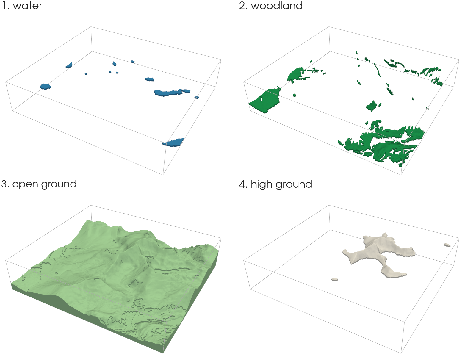
Mesh booleans can leave zero-volume slivers where two colour regions meet only at a corner. Here, 178 of them were attached to the open-ground body. They have no printable volume, but slicers report them as separate objects, so we drop any piece under 0.05 mm³. Then comes the proof that matters. Each part must be watertight and outward-facing, using the same edge checks as Part 1. The four volumes must add up to the whole terrain, and no two parts may overlap:
open ground dropped 178 slivers totalling 0.0000 mm3water 20,536 triangles | watertight True | oriented True | volume 0.49 cm3woodland 106,628 triangles | watertight True | oriented True | volume 2.39 cm3open ground 626,896 triangles | watertight True | oriented True | volume 257.33 cm3high ground 63,410 triangles | watertight True | oriented True | volume 1.96 cm3sum of parts 262.176 cm3 | whole terrain 262.176 cm3 | pairwise overlap -0.0005 mm3water 11 separate piece(s)woodland 65 separate piece(s)open ground 1 separate piece(s)high ground 3 separate piece(s)The parts sum to the terrain to the last cubic millimetre shown. The overlap is floating-point noise: half a thousandth of a cubic millimetre across all six pairs. The 11 water pieces and 65 woodland pieces are the separate lakes and woods; the open-ground body is one solid.
Step 5: STLs and a 3MF
Each part is written as a binary STL with the structured-dtype writer from Part 1. The four parts also go into one 3MF file: a zip containing an XML model, which keeps the parts together, named and in position, each with a display colour:
=== Step 5: write STLs and a 3MF ===yr_wyddfa_1_water.stl 1.0 MByr_wyddfa_2_woodland.stl 5.3 MByr_wyddfa_3_open_ground.stl 31.3 MByr_wyddfa_4_high_ground.stl 3.2 MByr_wyddfa_multicolour.3mf 7.4 MB | parts: water, woodland, open ground, high groundThe 3MF is less than a fifth of the size of the four STLs together, because it stores each shared vertex once and is zip-compressed.
Printing tips
- Loading the parts: select all four STLs and drag them into the slicer together. PrusaSlicer, Bambu Studio and OrcaSlicer ask whether to load them as one object with multiple parts; say yes, so they stay aligned. Then give each part its own filament.
- Choosing colours: high contrast reads best at this scale. A pale body with darker accents shows the woodland and lake shapes far better than four similar greens.
- Layer height: 0.2 mm is a good balance here. Thinner layers mean more layers, and on this model almost every layer has a swap, so print time and purge waste rise quickly.
- Purge: use your slicer’s “flush into infill” or “flush into object” option where available. With caps, the body is large enough to absorb much of the purge.
- Thin caps on steep slopes: the cap is 1.2 mm thick vertically, so on a steep face it is thinner when measured across the slope. If dark woodland shows through a pale cap on cliffs, raise
CAP_MMto 1.6 mm.
Limitations
- Land cover is a 10 m satellite classification. WorldCover marks tree cover and water well at this scale, but it is a model output with known errors. Treat the woodland outlines as indicative, not surveyed.
- Colour edges are pixel steps. Boundaries follow the 20 m grid, which gives a fine stair-step about 0.38 mm wide on the print. That is close to a nozzle width and rarely visible, but smoothing the polygons with
shapely’ssimplifybefore extruding would remove it. - The 700 m line is a pixel boundary. It follows the cells, not an interpolated contour, so it can differ from a mapped contour by up to half a cell (10 m).
Frequently asked questions
How do I 3D print a map in multiple colours?
Split the model into one watertight solid per colour, so that the parts fill the model exactly between them. Then load them into the slicer together as parts of one object and give each part a filament. A multi-material unit such as a Bambu Lab AMS or Prusa MMU swaps filament automatically. If your colours are only elevation bands, a single-extruder printer can do the same job with a filament change at the right layer height.
Should colours go all the way through a multi-colour print?
They do not have to. In this model, thin 1.2 mm colour caps over one body used 4.85 cm³ of accent filament instead of 59.18 cm³. They hardly changed the number of layers needing a filament swap (144 against 152 of 159). Use caps to save expensive filament, and use fewer colours or elevation bands to save swaps.
Why does my slicer show hundreds of tiny objects?
Mesh booleans can leave zero-volume slivers where two regions touch only at a corner. Decompose each part into connected pieces, drop any piece below a small volume (0.05 mm³ here), and union the rest. Removing specks with a sieve filter before cutting reduces the problem at source.
What is the smallest colour area I can print?
It depends on the nozzle, but a region a few nozzle widths across is a sensible minimum. With a 0.4 mm nozzle, about 1.2 × 1.2 mm, or 1.5 mm², works well. Set the threshold in millimetres on the print and convert it to cells for your print scale, as Step 2 does, so the clean-up stays right when you change the model size.
Can I use OpenStreetMap instead of WorldCover for water and woods?
Yes. Rasterise OSM natural=water and landuse=forest or natural=wood polygons onto the same grid with rasterio.features.rasterize, and use them in place of the WorldCover classes in Step 2. OSM edges are sharper, but coverage varies by area. Credit “© OpenStreetMap contributors” under the ODbL.
Next steps
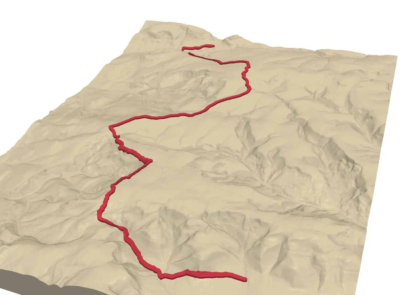
- Emboss a walking route in a contrasting colour: Part 2, GPX route on 3D-printed terrain, writes the route as its own part using the same boolean approach.
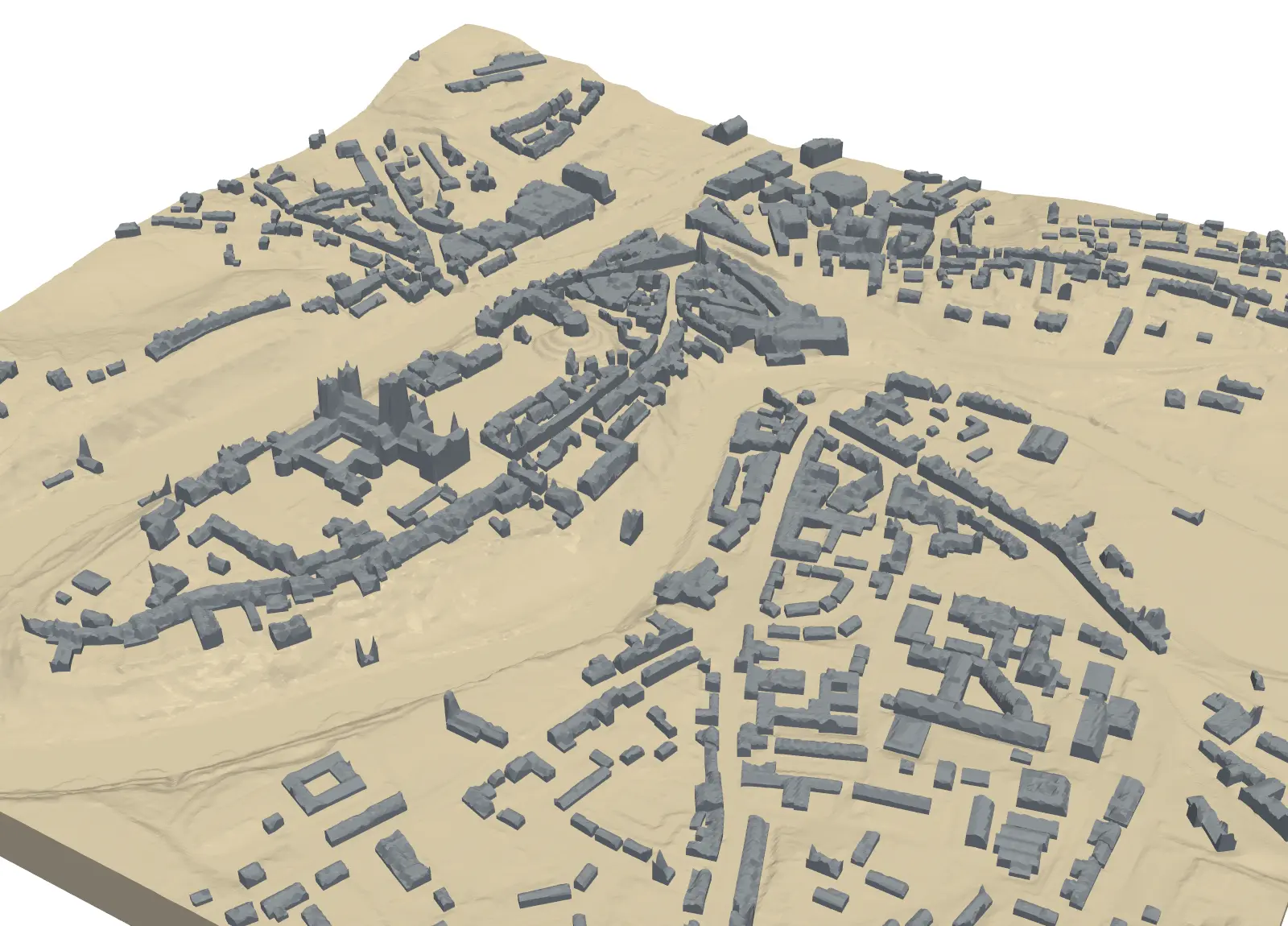
- Print a town instead of a mountain: Part 4, a 3D-printed city model, adds OpenStreetMap buildings to a LiDAR terrain, and buildings make an obvious second colour.
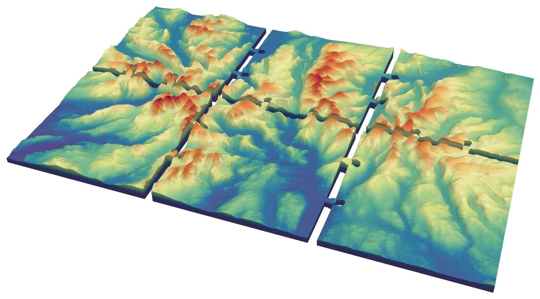
- Too big for your print bed? Part 5, tiling large regions, splits a region into jigsaw tiles, and the colour cut here works tile by tile.
- Preview the colours on screen first with 3D terrain visualisation with PyVista.
Data and licences
- Copernicus DEM GLO-30: © DLR e.V. 2010–2014 and © Airbus Defence and Space GmbH 2014–2018, provided under COPERNICUS by the European Union and ESA; all rights reserved. Accessed from the AWS Open Data registry.
- ESA WorldCover 10 m 2021 v200: © ESA WorldCover project 2021 / Contains modified Copernicus Sentinel data (2021) processed by ESA WorldCover consortium. Licensed under CC BY 4.0. Accessed from the AWS Open Data registry.
- Code:
multi_colour_terrain.py, tested with Python 3.12.0, numpy 2.5.4, rasterio 1.5.2, shapely 2.2.0, manifold3d 3.5.5 and pyvista 0.49.2. All processing runs locally; the only network requests read the two public rasters.
Key terms
- AMS / MMU
- Automatic Material System (Bambu Lab) and Multi Material Upgrade (Prusa): units that feed several filaments into one printer and swap between them during a print.
- Mesh boolean
- Union, difference or intersection of two closed solids. manifold3d performs these exactly and always returns a watertight result.
- Sieve filter
- A raster clean-up that replaces connected regions smaller than a size threshold with the value of their largest neighbour (rasterio.features.sieve).
- Purge or wipe tower
- A sacrificial block the printer extrudes into after each filament swap to flush the old colour out of the nozzle. Its size grows with the number of layers that change colour.
Data for this tutorial
- Copernicus DEM (GLO-30 / GLO-90) · Global 30 m elevation, free with attribution
- GIS data sources for the United Kingdom
Licences and formats for each source are listed in the GIS data sources catalogue.