Emboss a GPX route on 3D-printed terrain with Python: raised, engraved or two-colour inlay

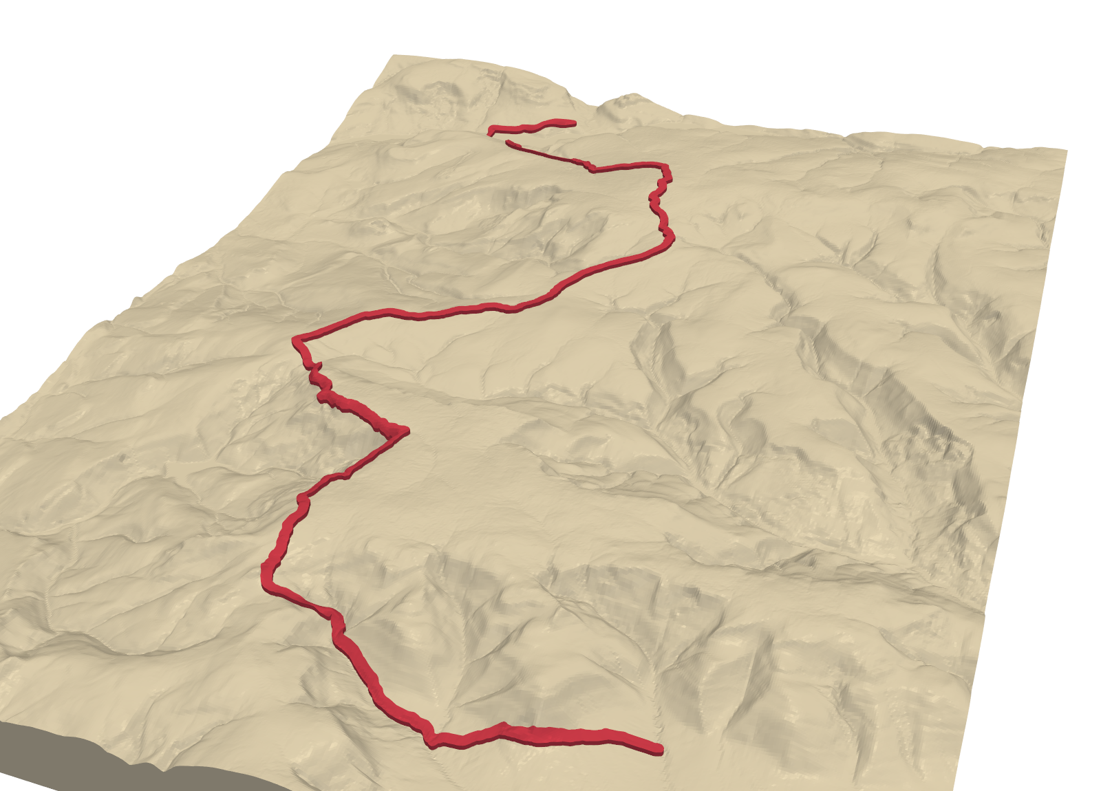
A terrain model with your own walk on it makes a good keepsake, and the route only needs a few lines of geometry. This tutorial takes a GPX track, drapes it on Environment Agency LiDAR terrain, and builds three printable versions: the route raised above the ground, engraved into it, and a two-colour inlay for a multi-material printer. The example is the first day of the Pennine Way, Edale to Crowden, over Kinder Scout and Bleaklow.

Part 1 of this series, From DEM to 3D-printable STL, built a terrain solid with NumPy. Here we reuse it and add the route with manifold3d, an exact mesh boolean library. The steps are:

1. read a GPX file and project it to British National Grid;
2. fetch the LiDAR terrain and average it to a printable grid;
3. drape the route and plot its elevation profile;
4. choose a scale and turn the route into a printable band;
5. build raised, engraved and inlay solids, and check each one;
6. write STLs and a 3MF.

The full script is gpx_route_terrain.py.

Step 1: read the route from GPX

Any GPX file from a watch, phone or route planner will do. A GPX file is plain XML, so the standard library can read it. This function takes the track points, or the route points if a planner wrote a route instead, from GPX 1.0 or 1.1:

def read_gpx(path):
    root = ET.parse(path).getroot()
    ns = root.tag[1:].split("}")[0] if root.tag.startswith("{") else ""
    q = (lambda t: f"{{{ns}}}{t}") if ns else (lambda t: t)
    pts = list(root.iter(q("trkpt"))) or list(root.iter(q("rtept")))
    return np.array([[float(p.get("lon")), float(p.get("lat"))] for p in pts])

lonlat = read_gpx(gpx_path)
to_bng = Transformer.from_crs("EPSG:4326", "EPSG:27700", always_xy=True)
E, N = to_bng.transform(lonlat[:, 0], lonlat[:, 1])
route = LineString(np.column_stack([E, N]))

So that the example runs for everyone, the script first builds a GPX file from the OpenStreetMap route relation for this stage of the Pennine Way, using the OSM API. It merges the relation’s 86 ways into one line and writes it out as a track. To use your own walk, point gpx_path at your file and change AOI to a box around it.

=== Step 1: the route as GPX ===
OSM relation 4080403: 'Pennine Way (Edale to Crowden)', 86 ways -> LineString
read pennine_way_edale_crowden.gpx: 1,733 track points
start 412,283 E 385,971 N | end 406,851 E 399,068 N | length 26.43 km
inside the model area: True

We ignore any elevations stored in the GPX. GPS heights are noisy, and the route must sit exactly on the printed surface, so its heights come from the same DEM as the terrain.

Step 2: LiDAR terrain at a printable resolution

The Environment Agency’s LiDAR composite DTM covers most of England at 1 m. That is far finer than a print at this scale can show: one millimetre on the model is about 94 m on the ground. We ask Defra’s Web Coverage Service (WCS) for 5 m cells, in 4 km tiles, and average each 5 × 5 block into one 25 m cell:

RES, FETCH = 25.0, 5.0
k = int(RES / FETCH)
# ... fill `fine` from twelve cached 4 km WCS tiles requested with SCALEFACTOR = 1 / FETCH
rows, cols = fine.shape[0] // k, fine.shape[1] // k
dem = np.nanmean(fine.reshape(rows, k, cols, k), axis=(1, 3))   # area mean, not point samples

Why not ask the WCS for 25 m cells directly? We tried. The service’s own downsampling repeated rows every four or five cells. That printed as fine terraces across the whole model, and it added false climbs to the profile. A block mean is honest: each cell is the average height of the 25 × 25 m it covers.

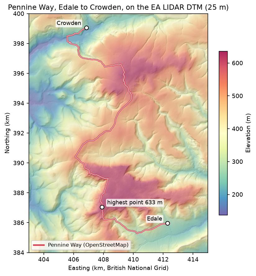
=== Step 2: Environment Agency LIDAR DTM, fetched at 5 m and averaged to 25 m ===
12 WCS tiles -> 2400 x 3200 cells of 5 m | no-data: 0
block mean 5 x 5 -> 480 x 640 cells of 25 m | empty cells filled: 0
elevation 137.7 - 635.8 m

Step 3: drape the route and plot the profile

To give the route heights, we walk along it every 25 m and sample the DEM with bilinear interpolation. scipy.ndimage.map_coordinates does that in one call, once the coordinates are converted to fractional rows and columns:

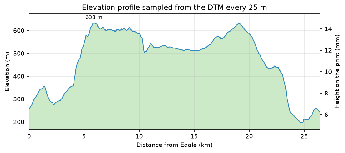
d = np.arange(0, route.length, RES)
pts = np.array([route.interpolate(s).coords[0] for s in d])
rc = np.vstack([(Y1 - pts[:, 1]) / RES - 0.5, (pts[:, 0] - X0) / RES - 0.5])
elev = ndimage.map_coordinates(dem, rc, order=1)

=== Step 3: drape the route on the DEM ===
sampled every 25 m: 1,058 points
lowest 197 m | highest 633 m at 5.9 km (407,902 E 387,059 N)
total ascent 817 m | total descent 830 m

The highest point, 633 m at 407,902 E 387,059 N, is beside the Kinder Low trig point. Total ascent depends on the resolution: a 25 m mean smooths out short ups and downs, so a GPS watch or a 1 m DEM will give a larger figure for the same walk. When the 25 m grid came straight from the WCS, with its repeated rows, the same calculation gave 936 m.

Step 4: scale and a printable route band

The model’s long side is set to 170 mm, which fixes the scale. The route is then drawn at a printable width rather than its true width. A footpath a metre or two wide would vanish at this scale, so we use 1.2 mm, three 0.4 mm extrusion lines:

scale = MODEL_LONG_MM / ((max(rows, cols) - 1) * RES)          # mm per metre
route_mm = LineString(to_mm(np.array(route.coords))).simplify(0.02)
band = route_mm.buffer(ROUTE_WIDTH_MM / 2, quad_segs=6).intersection(box(0.5, 0.5, W_mm - 0.5, D_mm - 0.5))

=== Step 4: model scale ===
horizontal scale 1:93,971 | cell on the print 0.266 mm
model 127.4 x 170.0 x 14.6 mm | route 1.2 mm wide = 113 m on the ground
route line: 1,733 -> 808 vertices after a 0.02 mm simplify
route outline: Polygon with 2,391 vertices, 0 holes, area 332.7 mm2

The band is clipped 0.5 mm inside the model edge so it never touches the side walls. Simplifying by 0.02 mm, a twentieth of a nozzle width, more than halves the vertex count with no visible change. The buffered band is a single polygon with no holes. If your route crosses itself, a loop or a there-and-back, the band will have holes, and the code handles those too.

Step 5: raised, engraved and inlay solids

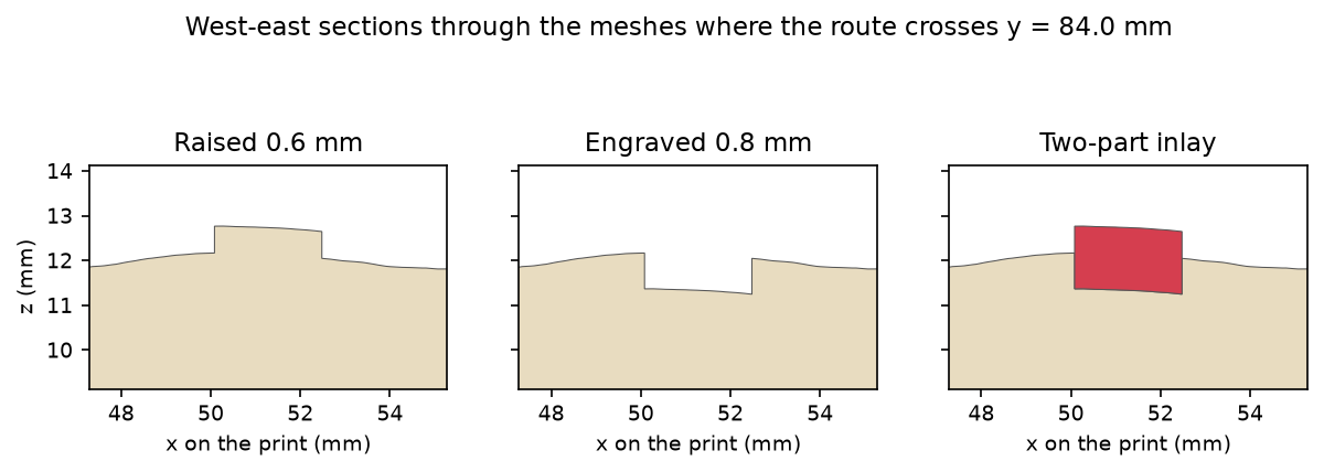
The trick is to cut the route against copies of the terrain shifted up or down, so that the route follows the slope. We build three terrain solids, at the surface, 0.6 mm above it and 0.8 mm below it. We also extrude the band into a tall prism:

terrain = to_manifold(*heightfield_solid(Z, cell_mm))
terrain_up = to_manifold(*heightfield_solid(Z + RAISE_MM, cell_mm))
terrain_down = to_manifold(*heightfield_solid(Z - DEPTH_MM, cell_mm))
prism = mf.Manifold.extrude(mf.CrossSection(contours), Z.max() + 10).translate((0, 0, -5))

ribbon = prism ^ terrain_up                           # the route column, cut off 0.6 mm above the surface
raised = terrain + ribbon                             # single colour, route stands proud
engraved = terrain - (prism - terrain_down)           # single colour, 0.8 mm groove
inlay = ribbon - terrain_down                         # second body that fills the groove

In manifold3d, + is union, - is difference and ^ is intersection. The inlay is the ribbon with everything below the groove floor removed. It fills the groove exactly and stands 0.6 mm proud, like the raised version. Each result is converted back to arrays and checked: every edge must be shared by exactly two triangles, in opposite directions.

=== Step 5: raised, engraved and inlay solids ===
terrain      1,228,796 triangles | watertight True | oriented True | volume  213.00 cm3
raised       1,259,666 triangles | watertight True | oriented True | volume  213.20 cm3
engraved     1,258,028 triangles | watertight True | oriented True | volume  212.74 cm3
route inlay     46,084 triangles | watertight True | oriented True | volume    0.47 cm3
[booleans and checks: 2.7 s]
engraved + inlay = 213.204 cm3 | raised = 213.204 cm3 | overlap between the two parts 0.0000 mm3
raised - terrain = 199.6 mm3 (route area 332.7 mm2 x 0.6 mm = 199.6 mm3)
route inlay: 1 piece(s)

All four solids are watertight and oriented. Two checks show the geometry is right as well as valid. The engraved terrain plus the inlay equals the raised model, with no overlap, so the two parts fit perfectly. And the raised model gains exactly the route area times 0.6 mm.

Step 6: STLs and a 3MF

=== Step 6: write STL and 3MF ===
pennine_way_raised.stl         63.0 MB | 1,259,666 facets | 84 + 50 x facets = file size: True
pennine_way_engraved.stl       62.9 MB | 1,258,028 facets | 84 + 50 x facets = file size: True
pennine_way_route_inlay.stl     2.3 MB | 46,084 facets | 84 + 50 x facets = file size: True
pennine_way_inlay.3mf          11.5 MB | parts: terrain, route

A binary STL is an 80-byte header, a 4-byte count and 50 bytes per triangle, so checking the file size against the count proves each file was written completely. The 3MF holds the engraved terrain and the inlay as two named parts in position, ready to assign to two filaments.

Which version to print

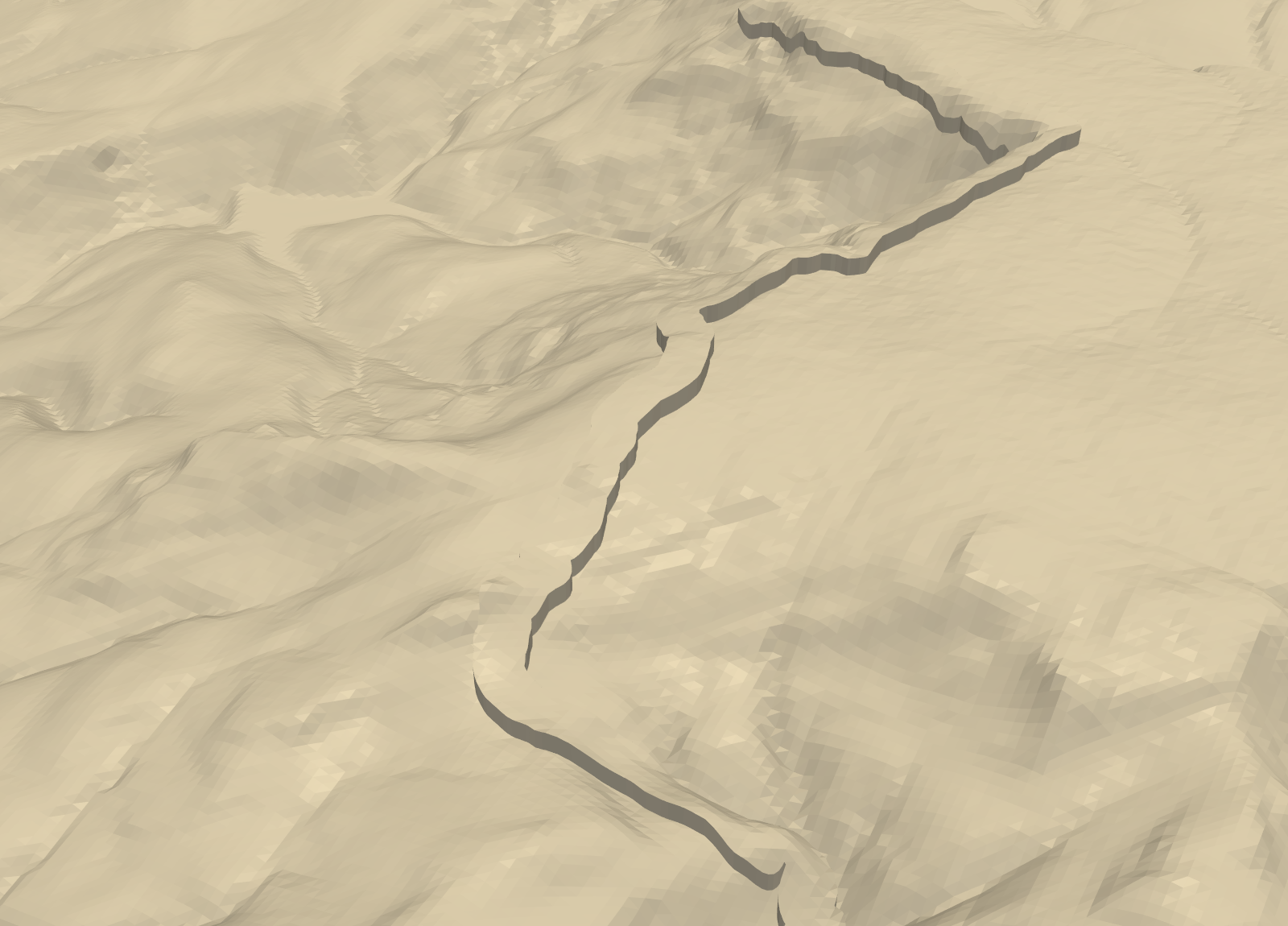
• Raised prints on any printer in one colour. It is the easiest to see from a low angle, and the route’s sharp edges show clearly.
• Engraved also prints in one colour, and you can fill the groove afterwards with paint or a paint pen.
• Inlay needs a multi-material printer, or a manual filament change. Because the inlay stands proud of the surface, the colour change starts at a different height on each part of the route. A single filament swap at one height will not separate it, so use an AMS, MMU or tool changer.

Printing tips

• Load both parts together. Open the 3MF, or select both STLs and load them as one object with multiple parts. The slicer keeps them aligned so you can give each part its own filament.
• Width: at least two or three line widths. Below about 0.8 mm the slicer may drop parts of the route altogether.
• Layer height: 0.2 mm or less, so the 0.6 mm rise is at least three layers.
• Ironing on the top surface can make a raised route stand out more cleanly, but it adds time on a large model.

Limitations

• The route is drawn wider than life. At 1.2 mm, the band covers 113 m on the ground, so it will hide small features close to the path, such as narrow cloughs.
• Ascent depends on resolution. The total ascent from a 25 m average is lower than you would get from a 1 m DTM or a GPS track. Use the profile for shape, not for official route statistics.
• LiDAR coverage is England only. Defra’s composite DTM covers England. For Wales, Scotland or elsewhere, use Copernicus GLO-30 or a national LiDAR product; the rest of the code is unchanged.

Frequently asked questions

How do I 3D print a hiking route on a map?

Read the GPX track, project it to the same grid as a DEM, and buffer it into a band a few nozzle widths wide. Then cut that band against the terrain solid with mesh booleans to raise or engrave it, as this tutorial does with manifold3d. Check the meshes are watertight before you slice them.

How wide should a route be on a 3D-printed map?

At least two nozzle widths, and preferably three: 1.2 mm with a 0.4 mm nozzle. Thinner lines may be dropped or printed patchily by the slicer. The route will be wider than life at most map scales, which is what makes it visible.

Can I use the elevations in my GPX file?

You can, but it is better not to. GPS heights are noisy and will not match the DEM surface, so the route would float above or sink into the terrain. Sampling heights from the DEM makes the route follow the printed surface exactly.

Can I print the route in a different colour on a single-extruder printer?

Only partly. A filament change at one height will not separate a route that climbs and descends with the terrain. Engrave it instead and fill the groove with paint, or use the raised version and paint the top of the ridge.

Where can I get a GPX file of a National Trail?

Many route planners can export GPX, and the National Trails website publishes routes for England and Wales. OpenStreetMap also maps most long-distance paths as route relations; this script builds a GPX file from one, and the same code works for any relation number.

Next steps

• Print the route in colour alongside woodland and water: Part 3, multi-colour terrain prints, splits terrain into one watertight part per colour.
• Too long for one print bed? Part 5, tiling large regions, splits a model into jigsaw tiles.
• Explore a track on screen first with Visualising a cycle track in 3D or 3D terrain visualisation with PyVista.
• Add the buildings of a town to the terrain with Part 4, a 3D-printed city model.
• New to the series? Part 1, From DEM to 3D-printable STL, builds the terrain solid used here.

Data and licences

• Environment Agency LiDAR Composite DTM (1 m): © Environment Agency copyright and/or database right. Contains public sector information licensed under the Open Government Licence v3.0. Accessed through the Defra Data Services Platform WCS.
• Route: Pennine Way (Edale to Crowden), OpenStreetMap relation 4080403. © OpenStreetMap contributors, available under the Open Database Licence. Any model printed from it should carry the same credit.
• Code: gpx_route_terrain.py, tested with Python 3.12.0, numpy 2.5.4, rasterio 1.5.2, shapely 2.2.0, manifold3d 3.5.5 and pyvista 0.49.2. All processing runs locally; the only network requests fetch the route from the OSM API and the terrain tiles from the WCS.