GPS data analysis in Python with MovingPandas: trajectories, speed, stops, generalisation and flow maps
A MovingPandas tutorial on one day of real AIS vessel tracks in Puget Sound: 277,574 GPS fixes from 703 vessels turned into trajectories, with speed and direction, outlier cleaning, stop detection at ferry terminals, splitting into 148 trips, Douglas-Peucker against time-aware generalisation, a flow map of 319 aggregated flows, and reading and writing GPX.
- Level
- Intermediate
- Tested with
- Python 3.12
- Source code
- Download scripts
Key takeaways
- `mpd.TrajectoryCollection(points, 'MMSI', t='t', min_length=1000)` turned 277,574 AIS fixes into 364 vessel trajectories in 1.0 s; splitting at 15-minute gaps in reception gave 403.
- Speed computed from positions with `add_speed()` matched the speed the ferry itself reported (median difference 0.50 km/h), but four bad fixes implied up to 58.8 km/h until `OutlierCleaner` removed them.
- `TrajectoryStopDetector` found 149 stops for seven Washington State Ferries, and they cluster exactly on the six terminals; `StopSplitter` cut the same tracks into 148 trips, 44 of them Bainbridge Island to Seattle with a median crossing of 30 minutes.
- Douglas-Peucker at 50 m kept 18% of the fixes, but the simplified ferry was on average 184 m from where it really was at the same moment. The time-aware top-down time ratio algorithm at the same tolerance kept 25% with a mean timing error of only 7 m.
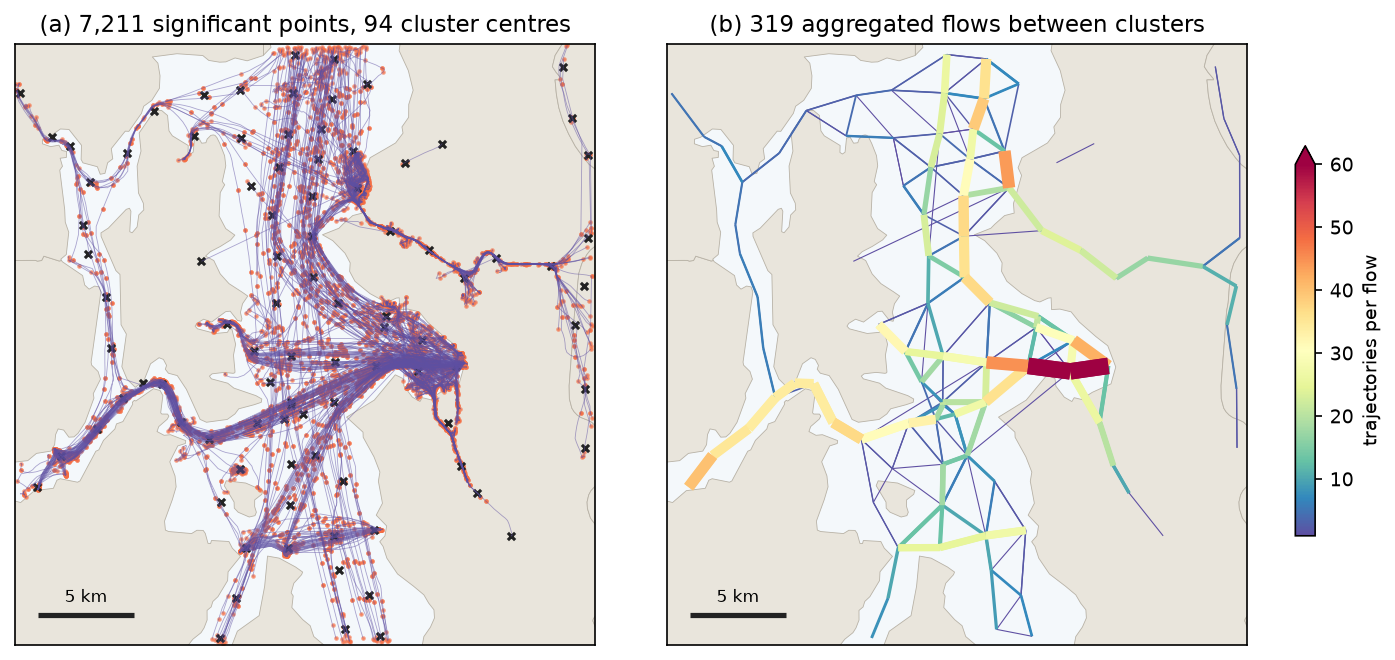
- `TrajectoryCollectionAggregator` summarised 253 moving vessels as 94 clusters and 319 flows; the strongest flow carried 108 trajectories.
Before you start
- Comfort with GeoPandas GeoDataFrames and projected coordinates; the coordinate reference systems tutorial covers why distances need metres
- Python 3.10+ with movingpandas, geopandas, shapely, pyproj, pandas, matplotlib, requests and gpxpy
- About 400 MB of free disk space and an internet connection: the script downloads one day of NOAA AIS (about 345 MB zipped) and a Census land layer, with no account or key
Short answer: to analyse GPS data in Python, load the fixes into a GeoDataFrame with a timestamp column, project them to metres, and build trajectories with MovingPandas: mpd.TrajectoryCollection(gdf, "track_id", t="time"). From there, add_speed() and add_direction() add movement attributes, OutlierCleaner removes impossible jumps, TrajectoryStopDetector finds stops, StopSplitter and ObservationGapSplitter cut tracks into trips, DouglasPeuckerGeneralizer or the time-aware TopDownTimeRatioGeneralizer simplify them, and TrajectoryCollectionAggregator turns many tracks into a flow map. GPX files from phones, watches and bike computers load with gpd.read_file(path, layer="track_points") and go through exactly the same steps.
A pile of GPS points is not yet movement data. The points need ordering by time and grouping by object before you can ask how fast something went, where it stopped, which route it took or where traffic concentrates. MovingPandas, built on GeoPandas, does that bookkeeping for you.
This tutorial uses one full day of real GPS tracks: AIS broadcasts from ships in central Puget Sound, Washington, on 1 June 2023. AIS is GPS with an identity attached. Every vessel reports its position, speed and heading, and NOAA publishes the archive as public domain data. The area is busy with Washington State Ferries, which make the results easy to check: the stops should be at ferry terminals, and the trips should match published crossing times.
You will:
- read 277,574 fixes and build trajectories;
- compute speed and direction, and check them against what the ships reported;
- clean out impossible fixes;
- detect stops;
- split tracks into trips;
- compare Douglas-Peucker with time-aware generalisation;
- aggregate everything into a flow map;
- write a trip to GPX and read it back.
Every number comes from gps_trajectories.py, which you can download with its pinned requirements.
Set up
Create a virtual environment and install the pinned versions:
python -m venv .venv.venv\Scripts\activate # macOS/Linux: source .venv/bin/activatepip install -r requirements.txt # movingpandas 0.23.0, geopandas 1.2.0, gpxpy 1.6.2, ...python gps_trajectories.pyThe first run downloads AIS_2023_06_01.zip (about 345 MB, the whole US coast for one day) and keeps only the central Puget Sound box in a small CSV, so later runs start in a fraction of a second.
Step 1: read GPS fixes and build trajectories
MarineCadastre distributes AIS as one CSV per day, with one row per position report. The important columns are the vessel identifier (MMSI), the timestamp (BaseDateTime), latitude and longitude, and the speed and course over ground the ship’s own GPS reported (SOG, in knots, and COG, in degrees). The script streams the national file in chunks of a million rows and keeps the box from Bremerton to Seattle and Vashon Island:
BBOX = (-122.65, 47.47, -122.25, 47.75)          # central Puget Sound: Seattle, Bainbridge, Bremerton, VashonUTM = 32610                                       # WGS 84 / UTM zone 10N, metres
with zipfile.ZipFile(zip_path) as z:    parts = []    for chunk in pd.read_csv(z.open(z.namelist()[0]), chunksize=1_000_000):        keep = chunk.LON.between(BBOX[0], BBOX[2]) & chunk.LAT.between(BBOX[1], BBOX[3])        parts.append(chunk[keep])pd.concat(parts).to_csv(cache, index=False)
ais = pd.read_csv(cache, parse_dates=["BaseDateTime"])ais = ais.drop_duplicates(["MMSI", "BaseDateTime"]).sort_values(["MMSI", "BaseDateTime"])pts = gpd.GeoDataFrame(ais, geometry=gpd.points_from_xy(ais.LON, ais.LAT), crs=4326).to_crs(UTM)AIS fixes in the Puget Sound box on 1 June 2023: 277,574 from 703 vessels (read in 0.1 s) MMSI BaseDateTime LAT LON SOG COG VesselName VesselType368252640 2023-06-01 00:00:02 47.72345 -122.64139 0.0 0.0 RUNRIG 37.0368028070 2023-06-01 00:00:05 47.64409 -122.34321 0.0 291.6 GRUMPYCAT 36.0367307370 2023-06-01 00:00:03 47.65774 -122.37130 0.0 1.4 NORTH AMERICAN 30.0duplicate timestamps dropped: 10time between fixes: median 179 s, 90th pct 240 s, max 21.3 hTwo preparation steps matter before anything else:
- Drop duplicate timestamps. Two fixes with the same time make speed infinite. There were only 10 here, but GPS logs and merged feeds often have more.
- Project to metres. MovingPandas measures length and speed in the units of the CRS when it is projected. UTM zone 10N gives metres; the coordinate reference systems tutorial explains how to choose a projection.
Now build the trajectories. One line groups the points by vessel and sorts them by time. min_length=1000 drops the 339 vessels that moved less than a kilometre all day, which are mostly boats tied up in marinas. A vessel that leaves the box and comes back hours later would otherwise be joined by a straight line across land, so ObservationGapSplitter breaks a trajectory wherever there is no fix for 15 minutes:
pts = pts.rename(columns={"BaseDateTime": "t"})tc = mpd.TrajectoryCollection(pts, "MMSI", t="t", min_length=1000)tc = mpd.ObservationGapSplitter(tc).split(gap=timedelta(minutes=15), min_length=1000)focus = next(tr for tr in tc if tr.df.VesselName.iloc[0] == "WSF WALLA WALLA")TrajectoryCollection: 364 trajectories longer than 1 km, built in 1.0 s (339 vessels moved less than 1 km and were left out)ObservationGapSplitter(gap=15 min): 403 trajectories after splitting at gaps in receptionWSF WALLA WALLA: 1 trajectory, 1,270 fixes, 282.1 km, 00:00 to 23:59 UTC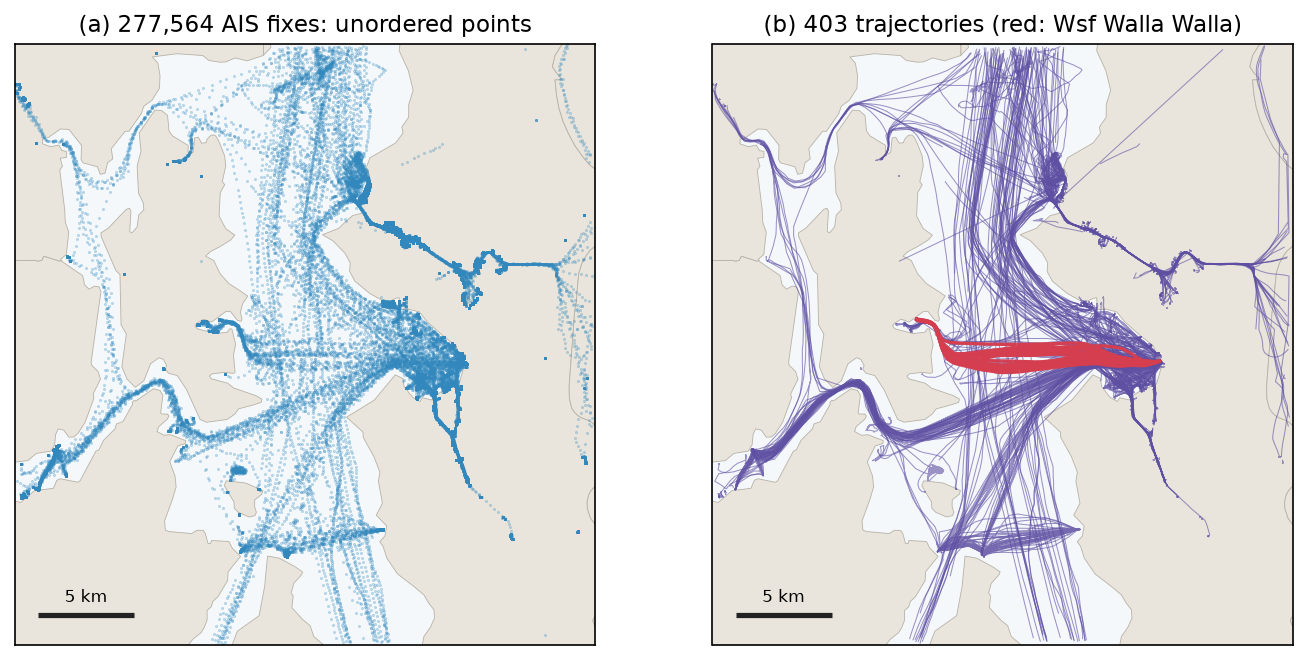
The ferry Walla Walla shuttled between Bainbridge Island and Seattle all day, covering 282 km in 1,270 fixes, about one fix every 68 seconds. That rate reflects the archive: MarineCadastre thins AIS to at most one fix per vessel per minute, and moored vessels report only every three minutes, which is why the median gap across all vessels is 179 s.
Step 2: speed and direction
add_speed() divides the distance between consecutive fixes by the time between them. add_direction() gives the bearing from each fix to the next, in degrees clockwise from north. AIS also carries the speed and course measured by the ship’s own GPS receiver, which makes a rare chance to check the computed values against an independent measurement:
focus.add_speed(overwrite=True, units=("km", "h"))focus.add_direction(overwrite=True)f = focus.dfsog_kmh = f.SOG * 1.852 # knots to km/hmoving = sog_kmh > 5diff = (f.speed - sog_kmh)[moving]ang = ((f.direction - f.COG + 180) % 360 - 180)[moving]WSF WALLA WALLA speed from positions vs reported SOG (moving fixes, n=541): median |difference| 0.50 km/h, r = 0.926direction from positions vs reported COG: median |difference| 1.2 degreesmax computed speed 58.8 km/h (31.8 kn); max reported SOG 18.1 knThe typical agreement is excellent: half a kilometre per hour and about one degree. The maximum is not. A ferry whose own GPS never reported more than 18.1 knots cannot have done 31.8 knots. A few fixes are displaced, and because speed is distance over a short time, one bad position creates two impossible speeds, one into it and one out of it. Figure 2 shows the spikes.
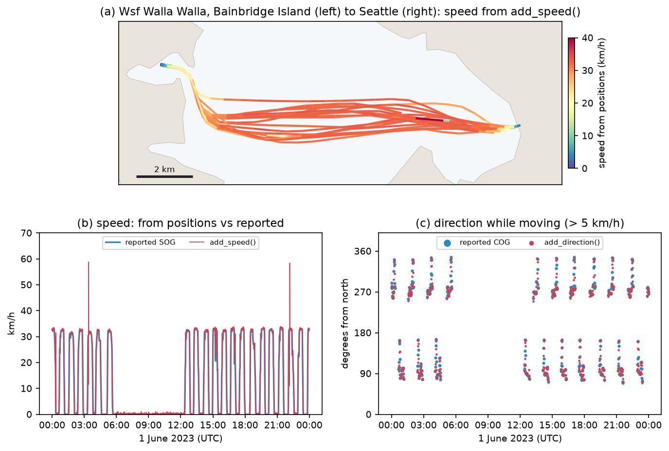
OutlierCleaner removes fixes that imply a speed above a threshold. Across all vessels, 100 km/h is a safe physical limit; for the ferry, 45 km/h is well above its 18-knot (33 km/h) service speed:
cleaned = mpd.OutlierCleaner(tc).clean(v_max=100, units=("km", "h"))focus_clean = mpd.OutlierCleaner(focus).clean(v_max=45, units=("km", "h"))fixes implying more than 100 km/h across all vessels: 3 in 3 trajectoriesOutlierCleaner(v_max=100 km/h) removed 3 fixesOutlierCleaner(v_max=45 km/h) on WSF WALLA WALLA: removed 4 fixes; max speed now 41.0 km/hThe remaining maximum of 41.0 km/h is still above the reported 33 km/h. Over a 60-second interval a position error of 100 m changes the computed speed by 6 km/h, so a few km/h of noise is normal for computed speeds. If your device records its own speed, as AIS, many sports watches and some GPX loggers do, prefer it for instantaneous speed and use positions for distances and averages.
Step 3: stop detection
A stop is a period in which the object stays inside a small circle for a minimum time. TrajectoryStopDetector takes both thresholds explicitly. Ferries sit at the berth for 10 to 25 minutes, so a 150 m diameter and a 5-minute minimum fit them; for a pedestrian or cyclist you might use 50 m and 2 minutes. The script runs the detector on the seven Washington State Ferries (WSF) in the box:
ferries = mpd.TrajectoryCollection([tr for tr in tc if str(tr.df.VesselName.iloc[0]).startswith("WSF ")])detector = mpd.TrajectoryStopDetector(ferries)stops = detector.get_stop_points(max_diameter=150, min_duration=timedelta(minutes=5))
# group the stop points into places: stops within 500 m of each other belong to the same terminalblobs = gpd.GeoDataFrame(geometry=list(stops.buffer(250).union_all().geoms), crs=UTM)blobs["place"] = range(len(blobs))stops = gpd.sjoin(stops, blobs, predicate="within").drop(columns="index_right")places = stops.dissolve("place", aggfunc={"duration_s": ["count", "median", "sum"]})
get_stop_points() returns one point per stop, with its start time, end time and duration_s. Grouping nearby stops, with a buffer and a spatial join, turns them into places, which the script then names from the nearest terminal:
Washington State Ferries in the box: 7 trajectories from Cathlamet, Chimacum, Kittitas, Samish, Sealth, Tacoma, Walla WallaTrajectoryStopDetector(max_diameter=150 m, min_duration=5 min): 149 stops in 1.1 sstop places (stops within 500 m grouped): name n_stops median_dwell_min hours_stopped lon lat Vashon 38 13.4 41.4 -122.4635 47.5111Seattle (Colman Dock) 31 20.5 11.3 -122.3402 47.6022 Fauntleroy 26 17.4 7.7 -122.3969 47.5232 Bainbridge Island 24 20.0 16.1 -122.5092 47.6221 Southworth 21 13.4 6.1 -122.4957 47.5132 Bremerton 8 16.6 6.8 -122.6247 47.5615 unnamed 1 1437.0 24.0 -122.3587 47.5873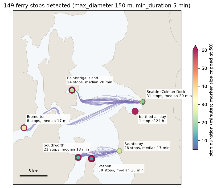
Every place is a ferry terminal, and the median dwell times of 13 to 21 minutes match ferry turnarounds. The detector also found something no timetable shows: one ferry never moved, and appears as a single stop of 24 hours at a lay-up berth near Harbor Island. Vashon’s 41.4 stop hours are far more than 38 stops of about 13 minutes would give, so a few ferries waited there for many hours outside the busiest periods. The median is the better summary of a normal turnaround.
Step 4: split tracks into trips
Most questions about movement concern trips: how long a crossing takes, or which route was used. StopSplitter uses the same stop definition to cut each trajectory at every stop, and min_length throws away the short pieces left by manoeuvring at the berth:
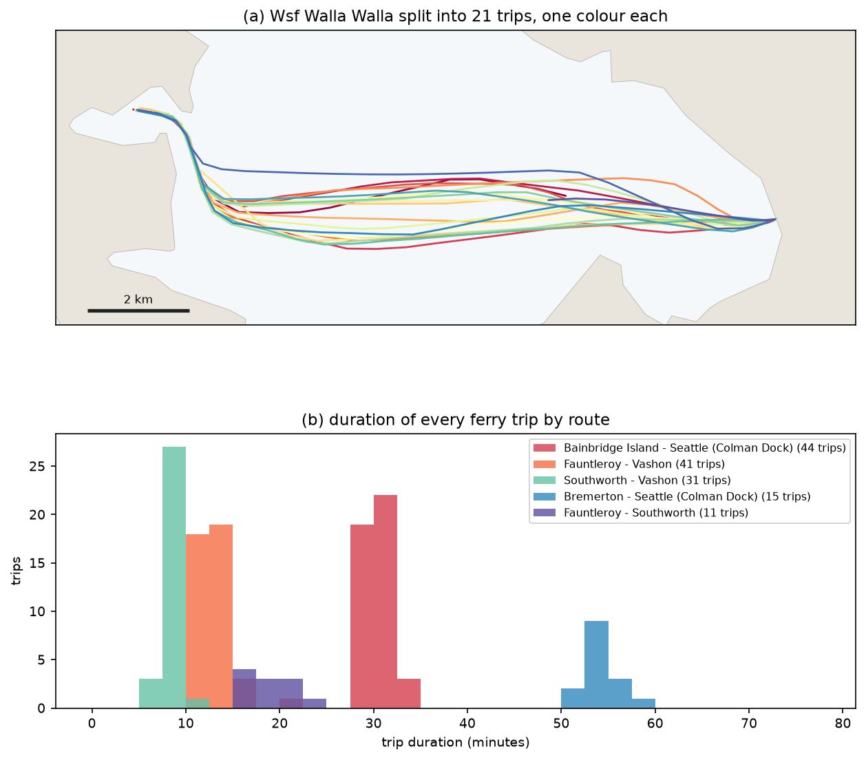
trips = mpd.StopSplitter(ferries).split(max_diameter=150, min_duration=timedelta(minutes=5), min_length=1000)for tr in trips: rows.append({"ferry": tr.df.VesselName.iloc[0].replace("WSF ", "").title(), "from": nearest_place(tr.get_start_location()), "to": nearest_place(tr.get_end_location()), "minutes": tr.get_duration().total_seconds() / 60, "km": tr.get_length() / 1000})StopSplitter(max_diameter=150 m, min_duration=5 min, min_length=1 km): 7 ferry trajectories -> 148 trips trips median_min median_kmrouteBainbridge Island - Seattle (Colman Dock) 44 30.3 13.7Fauntleroy - Vashon 41 12.7 5.2Southworth - Vashon 31 8.4 2.8Bremerton - Seattle (Colman Dock) 15 54.0 25.5Fauntleroy - Southworth 11 17.7 7.6Seattle (Colman Dock) - edge of box 3 12.1 5.6Bainbridge Island - edge of box 2 16.8 7.3Bremerton - edge of box 1 41.9 19.2WSF WALLA WALLA trips: 21, median crossing 29 min over 13.7 kmThe medians agree with the published crossing times of about 35 minutes for Seattle to Bainbridge and 60 minutes for Seattle to Bremerton, which include loading. The six “edge of box” trips are a reminder that analysis areas cut trips: those ferries left the box or arrived from outside it.
Other splitters in MovingPandas cut by time instead: TemporalSplitter by hour or day, ObservationGapSplitter at gaps (used in Step 1), SpeedSplitter when an object slows below a threshold for a while, and ValueChangeSplitter whenever a column such as a trip ID changes.
Step 5: generalisation, Douglas-Peucker against time-based
A day of one-minute fixes is more data than a map or a database often needs. Generalisation keeps a subset of the fixes. The classic algorithm, Douglas-Peucker, keeps the points needed to stay within a distance tolerance of the original line. It considers only shape. A ferry that slows down to dock follows a straight line, so Douglas-Peucker happily throws away every fix on the approach, and the simplified trajectory then claims the ferry moved at constant speed.
MovingPandas offers time-aware alternatives. The top-down time ratio (TDTR) algorithm measures the error to where the object should be at each timestamp, not to the nearest point of the line. MinTimeDeltaGeneralizer simply keeps one fix every so many minutes. To compare them fairly, the script measures two errors for every original fix:
- spatial error: the distance from the fix to the simplified line;
- synchronous error: the distance from the fix to where the simplified trajectory places the ferry at the same moment, by linear interpolation in time.
def errors(gen):    g = gen.df    gt = (g.index - fdf.index[0]).total_seconds().values    gx, gy = np.interp(tt, gt, g.geometry.x), np.interp(tt, gt, g.geometry.y)    sync = np.hypot(xy[:, 0] - gx, xy[:, 1] - gy)    spatial = shapely.distance(shapely.points(xy), gen.to_linestring())    return len(g), spatial, sync
for tol in [2, 5, 10, 20, 50, 100, 200, 400]: dp = mpd.DouglasPeuckerGeneralizer(focus).generalize(tolerance=tol) tdtr = mpd.TopDownTimeRatioGeneralizer(focus).generalize(tolerance=tol)mtd = mpd.MinTimeDeltaGeneralizer(focus).generalize(tolerance=timedelta(minutes=10))generalising WSF WALLA WALLA (1,266 fixes): method tolerance unit points kept_pct spatial_max_m spatial_mean_m sync_mean_m sync_max_m secs Douglas-Peucker 10.0 m 426 33.65 9.46 0.65 36.16 543.08 0.14 Douglas-Peucker 50.0 m 230 18.17 44.09 3.91 183.95 775.20 0.07 Douglas-Peucker 100.0 m 170 13.43 94.32 6.25 293.89 2399.97 0.07Top-down time ratio 10.0 m 571 45.10 9.22 0.38 2.39 9.85 0.92Top-down time ratio 50.0 m 314 24.80 40.11 2.96 7.17 49.84 0.63Top-down time ratio 100.0 m 233 18.40 95.27 4.34 16.43 98.35 0.74 Min. time delta 5.0 min 256 20.22 161.86 6.50 69.93 648.04 0.04 Min. time delta 10.0 min 137 10.82 333.46 12.65 202.45 1357.77 0.04At a 50 m tolerance both distance-based methods keep the shape to within about 40 to 45 m. The difference is in time. Douglas-Peucker kept 230 fixes but put the ferry on average 184 m, and at worst 775 m, from where it really was at that moment. TDTR kept 314 fixes and was never more than 50 m out, by construction. Keeping one fix every 10 minutes was the worst of all: 137 fixes, with corners cut by up to 333 m. Douglas-Peucker is about ten times faster, at 0.07 s against 0.63 s for TDTR, which only matters for millions of tracks.
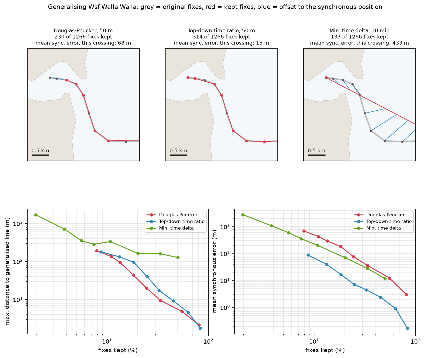
The rule of thumb: use Douglas-Peucker when you only need the route geometry, for example to draw a map or measure a path’s length. Use TDTR when the simplified data will be used for speeds, timings, interpolated positions or meeting points.
Step 6: aggregate trajectories into a flow map
With hundreds of trajectories, drawing every line hides the pattern. TrajectoryCollectionAggregator extracts significant points (starts, ends, stops and sharp turns), clusters them, and counts how many trajectories travel between each pair of clusters. The script first keeps the 253 trajectories that moved faster than 3 knots, and thins each one to a fix every 100 m so the clustering runs quickly:
movers = mpd.TrajectoryCollection([tr for tr in tc if tr.df.SOG.max() > 3])gen_tc = mpd.MinDistanceGeneralizer(movers).generalize(tolerance=100)agg = mpd.TrajectoryCollectionAggregator(gen_tc, max_distance=2000, min_distance=200, min_stop_duration=timedelta(minutes=5))sig = agg.get_significant_points_gdf()clusters = agg.get_clusters_gdf()flows = agg.get_flows_gdf() # LineStrings between cluster centres, with a 'weight' columnflow map from 253 vessels that moved faster than 3 kn: 7,211 significant points, 94 clusters, 319 flows in 9.2 sflow weights: median 5, max 108; flows with weight >= 5: 174max_distance sets the size of the clusters, here 2 km, and min_distance stops significant points within 200 m of each other from being counted twice. Smaller values give more, finer clusters and more flows.
Step 7: read and write GPX in Python
GPX is the XML format used by GPS watches, phones, bike computers and route planners. To write a trajectory as GPX, use gpxpy. GPX coordinates are always WGS 84 latitude and longitude, so convert back to EPSG:4326 first:
trip = ft.sort_values("minutes").iloc[len(ft) // 2].traj.to_crs(4326)gpx = gpxpy.gpx.GPX()track = gpxpy.gpx.GPXTrack(name=f"Wsf Walla Walla {trip.get_start_time():%Y-%m-%d %H:%M} UTC")gpx.tracks.append(track)seg = gpxpy.gpx.GPXTrackSegment()track.segments.append(seg)for t, p in zip(trip.df.index, trip.df.geometry): seg.points.append(gpxpy.gpx.GPXTrackPoint(p.y, p.x, time=t.to_pydatetime()))(OUT / "ferry_trip.gpx").write_text(gpx.to_xml(), encoding="utf-8")To read a GPX file into MovingPandas, open its track_points layer with GeoPandas. GDAL exposes GPX as several layers (waypoints, routes, tracks, route_points and track_points); only track_points keeps the timestamps:
gpx_pts = gpd.read_file("ferry_trip.gpx", layer="track_points")gpx_pts["time"] = pd.to_datetime(gpx_pts.time).dt.tz_localize(None)gpx_traj = mpd.Trajectory(gpx_pts.to_crs(UTM), traj_id="gpx", t="time")gpx_traj.add_speed(units=("km", "h"))wrote ferry_trip.gpx: 28 track points, 3.5 KBread back with geopandas (layer='track_points'): 28 rows, columns include ['track_fid', 'track_seg_point_id', 'time', 'geometry']GPX trajectory: 13.64 km in 0:29:24, max speed 33.0 km/h (original trip 13.64 km)gpxpy: Wsf Walla Walla 2023-06-01 15:48 UTC; first point 47.62192, -122.50777 at 2023-06-01 15:48:12; gpxpy length_2d 13.63 kmThe trip survives the round trip intact: 28 points, 13.64 km and 29 minutes 24 seconds. Its maximum speed of 33.0 km/h matches the ferry’s reported 18 knots. gpxpy.parse() is the alternative when you need GPX-specific fields such as elevation, heart rate extensions or several tracks in one file; its own length_2d() gives 13.63 km.
For a cycle ride, a run or a walk, the same steps apply: read track_points, project, build a Trajectory, then add speed, detect stops at cafés or junctions, and split into laps. The older tutorial on visualising a cycle track in 3D shows what to do with such a GPX track in ArcGIS Pro: draping it on terrain and drawing its elevation profile.
Caveats
- AIS is thinned and incomplete. MarineCadastre keeps at most one fix per vessel per minute, and reception from shore stations has gaps. Speeds between one-minute fixes smooth out acceleration, and stop durations are only accurate to about a minute. Small craft without AIS transponders are missing entirely.
- Computed speed is noisy. A single displaced fix produced a 58.8 km/h spike on a 33 km/h ferry. Clean outliers with a threshold based on the object’s physical limits, and prefer a device-reported speed for instantaneous values.
- Thresholds define the answer. Stops, trips and flows all depend on
max_diameter,min_duration, gap length and cluster distance. The values here suit ferries; walkers, cars and aircraft need their own, and they should be reported with the results. - Projection. UTM zone 10N is accurate here. For tracks that cross zones or continents, use a local projection per region, or let MovingPandas compute geodesic distances on unprojected WGS 84 data, which is slower.
- Edges of the analysis area. Clipping to a box creates trips that start or end at the edge (six here). Exclude them from duration statistics, or clip with a buffer.
- Flows are not routes. Aggregated flows are straight lines between cluster centres and can cross land.
Frequently asked questions
How do I analyse GPS data in Python?
Load the fixes into a GeoDataFrame with a timestamp and an object ID, drop duplicate timestamps, and project to a metric CRS. Then build trajectories with MovingPandas: mpd.TrajectoryCollection(gdf, "id", t="time"). Add speed and direction, clean outliers, and then detect stops, split trips or aggregate flows as your question requires. For one track, mpd.Trajectory(gdf, traj_id=1, t="time") does the same.
How do I read a GPX file in Python?
The quickest way is gpd.read_file("track.gpx", layer="track_points"), which returns a GeoDataFrame with one row per point and a time column, ready for MovingPandas. Use gpxpy.parse(open("track.gpx")) instead when you need the GPX structure itself: several tracks or segments, waypoints, elevation or sensor extensions. Both read WGS 84 coordinates.
What is MovingPandas used for?
MovingPandas adds a time dimension to GeoPandas. It handles trajectories of anything that moves, such as vehicles, ships, aircraft, animals, people or storms: computing speed, direction and acceleration, detecting stops, splitting and cleaning tracks, generalising them, and aggregating many tracks into flow maps. It works with any GPS-like data that has a position, a timestamp and an ID.
How do I calculate speed from GPS coordinates in Python?
Divide the distance between consecutive fixes by the time between them. In MovingPandas, traj.add_speed(units=("km", "h")) does this and handles units. Project to metres first, or MovingPandas will use geodesic distances. Expect noise: here computed speeds agreed with the ship’s own measurement to a median of 0.5 km/h, but a few bad fixes produced impossible spikes until OutlierCleaner removed them.
What is the difference between Douglas-Peucker and top-down time ratio?
Both keep the fewest points within a distance tolerance. Douglas-Peucker measures the distance from each point to the simplified line and ignores time. Top-down time ratio measures the distance to where the object would be at that point’s timestamp, so it keeps points where speed changes. In this tutorial, at 50 m, Douglas-Peucker’s mean timing error was 184 m and top-down time ratio’s was 7 m.
How do I detect stops in GPS data?
Use mpd.TrajectoryStopDetector(traj).get_stop_points(max_diameter=150, min_duration=timedelta(minutes=5)). It returns one point per period in which the object stayed within the given diameter for at least the given time, with start time, end time and duration. Choose the thresholds to suit the object and the fix rate. With one-minute fixes, stops shorter than a few minutes cannot be detected reliably.
Next steps
- Use DBSCAN spatial clustering in Python on stop points to find places without a list of terminals, a more general version of the buffer grouping used here.
- Detect ships that do not broadcast AIS in Sentinel-1 radar images with SAR ship detection using CFAR, and match detections to AIS tracks like these to find dark vessels.
- Count fixes or stops in hexagons with the H3 hexagon grid in Python, or smooth them into a density surface with kernel density estimation in Python.
- Put trajectories and stops on a zoomable web map with interactive web maps with Folium.
- Turn addresses into coordinates, the other common source of point data, with geocoding in Python.
Data and licences
- AIS vessel traffic data, 1 June 2023: Bureau of Ocean Energy Management (BOEM) and National Oceanic and Atmospheric Administration (NOAA), from MarineCadastre.gov. US government work, in the public domain. Accessed on 3 November 2026.
- 2023 cartographic boundary file, county subdivisions, Washington (1:500,000): US Census Bureau, from the cartographic boundary files. Public domain. Accessed on 3 November 2026.
- Code:
gps_trajectories.py, tested with Python 3.12.0, movingpandas 0.23.0, geopandas 1.2.0, shapely 2.2.0, pandas 3.1.0 and gpxpy 1.6.2.
Key terms
- Trajectory
- An ordered sequence of timestamped positions for one moving object. MovingPandas stores it as a GeoDataFrame of points indexed by time.
- AIS
- The Automatic Identification System: ships broadcast their GPS position, speed over ground (SOG), course over ground (COG) and identity (MMSI) every few seconds to minutes.
- Stop
- A period in which an object stays within a small area (here a 150 m diameter) for at least a minimum duration (here 5 minutes).
- Douglas-Peucker
- A line simplification algorithm that keeps only the points needed to stay within a distance tolerance of the original line. It ignores time.
- Top-down time ratio (TDTR)
- A time-aware version of Douglas-Peucker that measures the error to where the object should be at each timestamp, so it keeps the points where speed changes as well as direction.
- Synchronous error
- The distance between an original fix and the position the generalised trajectory gives for the same moment. It measures how well a simplified track preserves timing, not just shape.
- Flow map
- A map of movement between places, where many trajectories are aggregated into weighted links between clusters of significant points.
Data for this tutorial
- MarineCadastre.gov AIS · NOAA and BOEM vessel traffic, 1 June 2023, US coastal waters; the script keeps central Puget Sound
- US Census cartographic boundary files · 2023 county subdivisions for Washington (1:500,000), used as the land layer
Licences and formats for each source are listed in the GIS data sources catalogue.