Height above nearest drainage (HAND) flood mapping in Python: the River Severn
Compute height above nearest drainage (HAND) from the Environment Agency LIDAR DTM at 5 m with pysheds, turn it into inundation extents for a range of stage heights on the River Severn between Shrewsbury and Buildwas, relate them to the Buildwas gauge, and score them honestly against the Environment Agency Flood Map for Planning with the hit rate, false-alarm ratio and critical success index.
- Level
- Intermediate
- Tested with
- Python 3.12
- Source code
- Download scripts
Key takeaways
- HAND is the height of each DEM cell above the stream cell it drains to. Once the DEM is conditioned and a drainage network chosen, pysheds computes it in one call: grid.compute_hand(fdir, dem, streams).
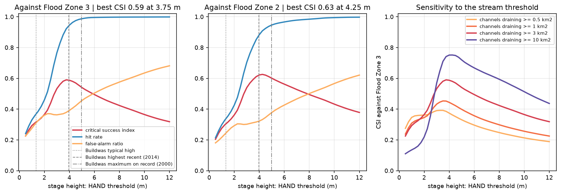
- Thresholding HAND at a stage height gives an inundation extent. On a 13 km × 10 km reach of the River Severn, HAND ≤ 3.75 m matched Environment Agency Flood Zone 3 with a critical success index of 0.59, a hit rate of 0.92 and a false-alarm ratio of 0.38.
- The drainage network matters as much as the stage. Drawing channels from 0.5 km² cut the best CSI to 0.39, and from 10 km² raised it to 0.75, because one HAND threshold assumes every small stream rises as far as the Severn.
- HAND has no hydraulics or flood volume. It overpredicts along small tributaries and on flat ground beside them, and underpredicts where the valley narrows and water stands deeper.
Before you start
- Watershed delineation with pysheds: conditioning a DEM, D8 flow direction and flow accumulation, as covered in the watershed delineation tutorial
- Python 3.10+ with pysheds, numba, numpy, scipy, rasterio, geopandas, shapely, pyproj, pandas, matplotlib and requests
- An internet connection: the DTM, flood zones and gauge data come from Environment Agency web services and the rivers from the OpenStreetMap Overpass API, with no accounts or keys
Short answer: height above nearest drainage (HAND) is the height of every DEM cell above the stream cell its water drains to. To compute it in Python, condition a DEM with pysheds, compute D8 flow direction and flow accumulation, and define a drainage network. Then call grid.compute_hand(fdir, dem, streams). For a simple flood map, every cell with HAND ≤ h is flooded at a stage height of h metres above the river. Always score the result against an independent flood map, for example with the critical success index (CSI).
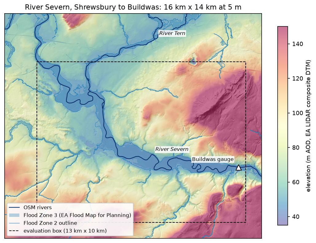
HAND is popular because it is fast and needs nothing but a DEM, which is why it underpins national-scale flood inundation mapping such as the NOAA Office of Water Prediction’s HAND-based system. However, it is a terrain index, not a flood model. In this tutorial we compute it from Environment Agency LIDAR for a 13 km reach of the River Severn between Shrewsbury and Buildwas in Shropshire. We map flood extents for a range of stage heights, and measure how well they agree with the Environment Agency’s own Flood Map for Planning.
You will learn how to:
- download the EA LIDAR Composite DTM at 5 m through its WCS;
- download Flood Zones 2 and 3 from the EA’s OGC API and rasterise them;
- burn mapped rivers into the DTM and route flow with pysheds;
- compute HAND and relate it to the Buildwas gauge;
- threshold HAND into inundation extents for several stage heights;
- score each extent against the flood zones with the hit rate, false-alarm ratio and CSI, and test the stream threshold.
All outputs below are real results from hand_flood_mapping.py, run on 3 November 2026 with Python 3.12, pysheds 0.5, numpy 2.5.4, rasterio 1.5.2 and geopandas 1.2.0. DEM conditioning and flow routing are covered in depth in watershed delineation in Python, so here we only adapt them for HAND.
Step 1: the LIDAR DTM
The Environment Agency’s LIDAR Composite DTM is a bare-earth model of England at 1 m, with buildings and vegetation removed. That makes it far better than a global surface model for floodplains, where a 2 m hedge or a block of trees changes everything. Its Web Coverage Service (WCS) can resample on the server. We ask for 2 km tiles with SCALEFACTOR=0.2, which returns 5 m cells and keeps the grid to a manageable 9 million cells:
RES = 5.0X0, Y0, X1, Y1 = 350_000, 300_000, 366_000, 314_000 # 16 km x 14 km, British National GridWCS = ("https://environment.data.gov.uk/spatialdata/lidar-composite-digital-terrain-model-dtm-1m/wcs?" "service=WCS&version=2.0.1&request=GetCoverage" "&CoverageId=13787b9a-26a4-4775-8523-806d13af58fc__Lidar_Composite_Elevation_DTM_1m" "&format=image/tiff&subset=E({},{})&subset=N({},{})&SCALEFACTOR={}")TILE = 2_000dtm = np.full((H, W), np.nan, dtype="float32")for ty in range(Y0, Y1, TILE): for tx in range(X0, X1, TILE): r = requests.get(WCS.format(tx, tx + TILE, ty, ty + TILE, 1 / RES), timeout=120) with rasterio.MemoryFile(r.content) as mem, mem.open() as src: tile = src.read(1).astype("float32") tile[(tile < -100) | (tile > 2000)] = np.nan # the WCS marks gaps with -3.4e38 row, col = rowcol(TRANSFORM, src.bounds.left + RES / 2, src.bounds.top - RES / 2) dtm[row:row + tile.shape[0], col:col + tile.shape[1]] = tile[:H - row, :W - col]DTM box 350000-366000 E, 300000-314000 N (16 km x 14 km) | 3200 x 2800 cells at 5 m | evaluation box 13 km x 10 kmelevation 22.5-406.7 m | gaps 0 cells (0.000%)The 56 tiles have no gaps in this area. The script still fills any gaps with the nearest valid value, because one hole in a floodplain breaks flow routing. All scores below use an evaluation box 1–2 km inside the DTM. Near the edge of a DEM, flow paths are cut off and HAND is unreliable.
Step 2: the reference flood zones, rivers and gauge
The Flood Map for Planning shows where flooding from rivers and the sea could happen if there were no defences. Flood Zone 3 has a 1% or greater chance of river flooding each year, and Flood Zone 2 a chance between 0.1% and 1%. The EA serves both through an OGC API Features endpoint that pages its results, so the script follows the next links:
FZ_URL = ("https://environment.data.gov.uk/geoservices/datasets/04532375-a198-476e-985e-0579a0a11b47/ogc/features/v1/" f"collections/Flood_Zones_2_3_Rivers_and_Sea/items?f=application/json&bbox={lon0},{lat0},{lon1},{lat1}&limit=200")feats, url = [], FZ_URLwhile url: page = requests.get(url, timeout=180).json() feats += page["features"] url = next((l["href"] for l in page.get("links", []) if l["rel"] == "next"), None)fz = gpd.GeoDataFrame.from_features(feats, crs=4326).to_crs(27700).explode(index_parts=False)fz = fz[fz.geom_type.isin(["Polygon", "MultiPolygon"])] # a few features arrive as mixed collectionsfz["geometry"] = fz.geometry.buffer(0).intersection(box(X0, Y0, X1, Y1))fz3_geom = fz[fz.flood_zone == "FZ3"].geometry.union_all()fz2_geom = fz[fz.flood_zone == "FZ2"].geometry.union_all()FZ3 = features.rasterize([(fz3_geom, 1)], out_shape=(H, W), transform=TRANSFORM, dtype="uint8").astype(bool)FZ2 = features.rasterize([(fz2_geom.union(fz3_geom), 1)], out_shape=(H, W), transform=TRANSFORM, dtype="uint8").astype(bool) # the Flood Zone 2 extent includes zone 319411 polygons | by zone and source: FZ2/river 17389, FZ3/river 2022FZ3 15.17 km2 | FZ2 polygons 3.52 km2, of which 0.00 km2 overlaps FZ3River Severn 30.8 km, River Tern 10.1 km, River Roden 2.7 km, unnamed 0.5 kmBuildwas gauge on the River Severn at 364570 E, 304420 N | gauge datum 36 m AOD | typical high 3.4 m | highest recent 6.025 m (2014-02-11) | maximum on record 7.037 m (2000-11-02)The Flood Zone 2 polygons do not overlap zone 3. They are only the extra fringe, so the full 0.1% extent is zone 2 plus zone 3. The script also downloads the rivers from OpenStreetMap and the Buildwas gauge record from the EA’s real-time flood-monitoring API: its datum, its typical high level, and the record levels of February 2014 and November 2000.
Step 3: burn the rivers and route the flow
HAND needs two things from flow routing: a D8 flow direction grid that says where each cell’s water goes, and a drainage network to measure heights against. The steps are the same as in watershed delineation: fill pits and depressions, resolve flats, then compute flow direction and accumulation. Two adaptations matter on a lowland floodplain.
First, burn the mapped rivers into a copy of the DTM. On a floodplain only a few metres of relief separate the river from the fields. Without burning, D8 flow can cut across meander necks and old channels instead of following the river. Second, round to 1 cm before conditioning. With sub-millimetre differences on flats, pysheds’ resolve_flats can leave cells that drain nowhere, and those cells get no HAND value. The LIDAR is only accurate to about 0.1 m vertically, so nothing is lost:
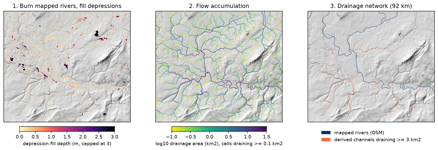
grid = Grid.from_raster(str(dem_path))dem = grid.read_raster(str(dem_path))river_px = features.rasterize([(g, 1) for g in rivers.values()], out_shape=(H, W), transform=TRANSFORM, dtype="uint8").astype(bool)burned = Raster(np.round(np.where(river_px, np.asarray(dem) - 5.0, np.asarray(dem)).astype("float64"), 2), viewfinder=grid.viewfinder) # for routing onlypit_filled = grid.fill_pits(burned)flooded = grid.fill_depressions(pit_filled)inflated = grid.resolve_flats(flooded)fdir = grid.flowdir(inflated, dirmap=DIRMAP)acc = grid.accumulation(fdir, dirmap=DIRMAP)burned 8,039 river cells by 5 m | 0 unresolved interior pits | fill, resolve flats, D8 and accumulation in 11.6 s | 6.0% of cells raised by depression filling, deepest fill 82.1 mWith the rounding, no interior pits remain. The deepest fill, 82 m, is a closed hollow in the north-east of the box, well away from the rivers.
Choosing the drainage network
This is the most important decision in HAND mapping. A 16 km DTM cannot see the roughly 2,000 km² the Severn drains before it enters the box. Accumulation alone would therefore not call the Severn a river until well downstream. The network is the mapped rivers plus every derived channel that drains at least 3 km² inside the box. The Flood Map for Planning’s river modelling generally covers watercourses with catchments of about 3 km² or more, so this threshold compares like with like:
acc_km2 = np.asarray(acc) * RES ** 2 / 1e6BOOL_VF = ViewFinder(affine=grid.affine, shape=grid.shape, crs=grid.crs, nodata=False)   # for mask rastersSTREAM_KM2 = 3.0
def hand_for(threshold_km2):    streams = (acc_km2 >= threshold_km2) | river_px    h = grid.compute_hand(fdir, dem, Raster(streams, viewfinder=BOOL_VF), dirmap=DIRMAP)    return streams, np.asarray(h, dtype="float64")
streams, hand_raw = hand_for(STREAM_KM2)streams draining >= 3 km2: 18,304 cells, about 92 km of channel | HAND computed in 1.3 sNote that compute_hand takes the unburned dem. The burned and filled copy only decides where water goes. Heights are measured on the real ground surface.
Step 4: height above nearest drainage
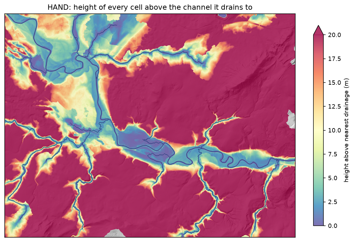
pysheds traces each cell’s D8 flow path down to the first stream cell, and subtracts that cell’s elevation from its own. A few cells sit below their drainage cell, because they are in filled hollows. These are clipped to zero. Cells whose flow path leaves the grid before it meets a channel have no HAND value, and are treated as dry:
hand = np.where(np.isfinite(hand_raw), np.clip(hand_raw, 0, None), np.nan)evaluation box: 5,200,000 cells, 20,946 without a HAND value (they drain off the grid before meeting a channel and count as dry)HAND percentiles 10/25/50/75/90: 2.9 / 10.6 / 26.7 / 47.4 / 81.7 m | 0.39% of cells sit below their drainage cell (set to 0) Flood Zone 3 11.28 km2 | median HAND 2.2 m | 90th percentile 3.6 m Flood Zone 2 13.44 km2 | median HAND 2.3 m | 90th percentile 4.1 m outside Flood Zone 2 116.04 km2 | median HAND 29.9 m | 90th percentile 86.1 mThis is the first sign that HAND works here. Nine-tenths of Flood Zone 3 lies within 3.6 m of its drainage, while the median HAND outside the flood zones is 29.9 m.
HAND and the Buildwas gauge
A HAND threshold is a height above the river surface as it was during the LIDAR survey, not above the gauge datum. To relate them, the script finds the lowest stream cell near the gauge and converts the gauge’s levels into heights above that surface:
LIDAR water surface at Buildwas 38.06 m AOD = stage 2.06 m on the gauge typical high stage 3.40 m -> 1.34 m above the LIDAR water surface highest recent (2014) stage 6.03 m -> 3.96 m above the LIDAR water surface maximum on record (2000) stage 7.04 m -> 4.98 m above the LIDAR water surfaceOn the day of the survey the Severn at Buildwas stood at a stage of about 2.06 m. The February 2014 flood peaked about 4 m above that, and the November 2000 flood, the highest on record, about 5 m above it. These heights apply at Buildwas only. Upstream the water surface is higher, but because HAND is measured from the local channel, a single threshold is still a fair first approximation along one reach.
Step 5: inundation extents for several stage heights
An inundation extent for a stage height h is simply hand <= h. The script steps h from 0.5 m to 12 m and scores each extent against the reference inside the evaluation box. Hits (a) are flooded in both, false alarms (b) only in HAND, and misses (c) only in the reference:
def scores(pred, ref, mask):    a = (pred & ref & mask).sum(); b = (pred & ~ref & mask).sum(); c = (~pred & ref & mask).sum()    return {"area_km2": (pred & mask).sum() * RES ** 2 / 1e6, "hit": a / (a + c), "far": b / (a + b),            "csi": a / (a + b + c), "bias": (a + b) / (a + c)}
STAGES = np.round(np.arange(0.5, 12.01, 0.25), 2)table = {z: [scores(hand <= h, ref, ev) for h in STAGES] for z, ref in (("FZ3", FZ3), ("FZ2", FZ2))}
The critical success index is the standard score for flood maps. It ignores the correctly dry cells, which make up most of any map and would otherwise inflate the accuracy. A map that floods everything has a hit rate of 1 but a poor CSI. For more on agreement measures, see land-cover accuracy assessment in Python.
stage | area km2 | FZ3 hit FAR CSI | FZ2 hit FAR CSI 1.0m | 5.13 | 0.33 0.27 0.29 | 0.30 0.22 0.28 2.0m | 8.09 | 0.46 0.36 0.37 | 0.43 0.29 0.36 3.0m | 13.56 | 0.77 0.36 0.53 | 0.70 0.30 0.54 4.0m | 17.53 | 0.95 0.39 0.59 | 0.88 0.32 0.62 5.0m | 20.46 | 0.99 0.46 0.54 | 0.95 0.38 0.60 6.0m | 22.65 | 1.00 0.50 0.49 | 0.97 0.43 0.56 7.0m | 24.64 | 1.00 0.54 0.46 | 0.98 0.47 0.53 8.0m | 26.53 | 1.00 0.58 0.42 | 0.98 0.50 0.49 10.0m | 30.83 | 1.00 0.63 0.36 | 0.99 0.57 0.43 12.0m | 35.38 | 1.00 0.68 0.32 | 1.00 0.62 0.38best match to FZ3: HAND <= 3.75 m | CSI 0.59 | hit rate 0.92 | false-alarm ratio 0.38 | bias 1.48 | 16.74 km2 (reference 11.28 km2)best match to FZ2: HAND <= 4.25 m | CSI 0.63 | hit rate 0.91 | false-alarm ratio 0.33 | bias 1.36 | 18.30 km2 (reference 13.44 km2)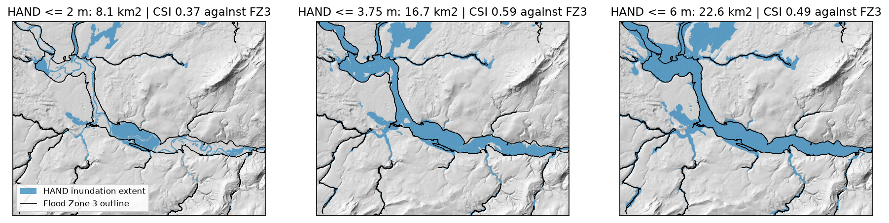
The best match to Flood Zone 3 is HAND ≤ 3.75 m, with a CSI of 0.59. It finds 92% of the zone, but 38% of what it floods lies outside it. Above 4 m the hit rate barely rises, while false alarms keep growing. Against the larger 0.1% extent, the best threshold rises to 4.25 m, as you would expect for a rarer flood. The best-fitting stage for Flood Zone 3, 3.75 m, is close to the 2014 flood at Buildwas (3.96 m). That is a reassuring check, but only a rough one: the 2014 flood was not a 1% event at every point of the reach.
Step 6: where it agrees, and the stream threshold
The agreement map shows where the errors are:
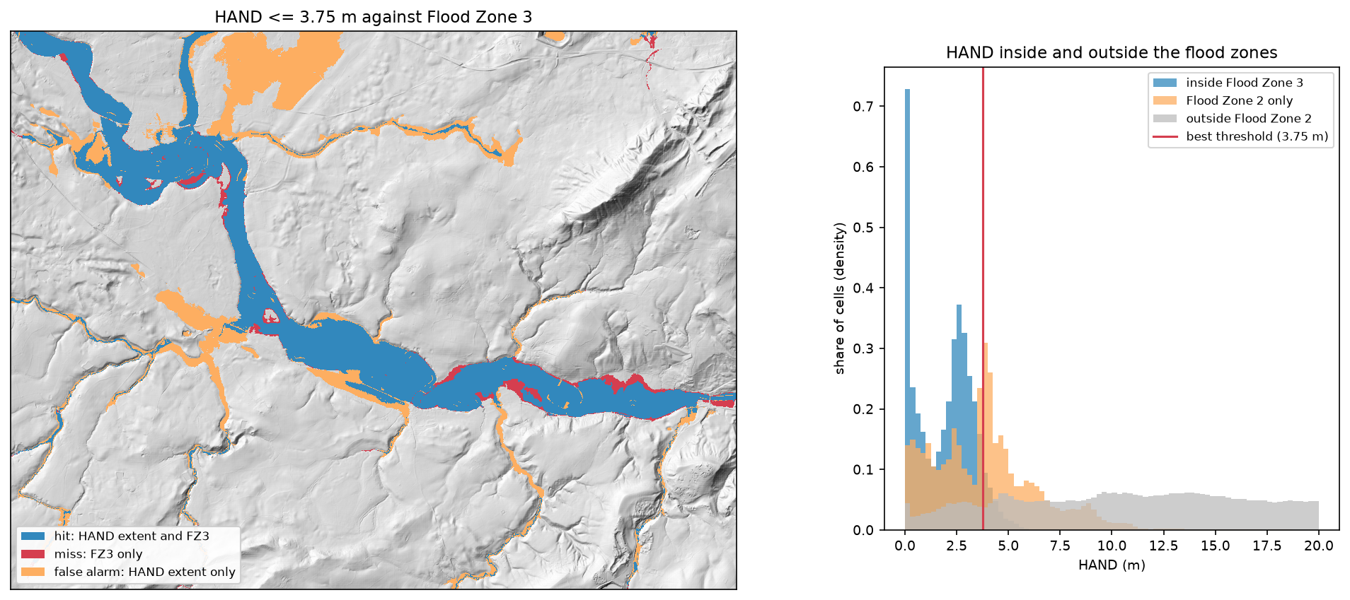
- Hits cover the Severn and Tern floodplains. Along the main rivers, HAND and the EA’s hydraulic modelling largely agree.
- False alarms line almost every tributary, and cover a large area of flat ground in the north, beside the Tern. A single threshold assumes every channel rises 3.75 m in a flood. The Severn does, but a stream draining 5 km² rises perhaps a metre. Flat ground beside a small derived channel can be low in HAND even though a flood never reaches it.
- Misses cluster along the southern edge of the Severn floodplain towards Buildwas, and in a few meander loops downstream of Shrewsbury. Where the valley narrows, water stands deeper for the same flow, so a single threshold is too low.
If small streams cause most false alarms, the channel threshold should matter, and it does:
streams >= 0.5 km2: 224 km of channel | best FZ3 CSI 0.39 at HAND <= 3.25 m | false-alarm ratio 0.59streams >= 1.0 km2: 160 km of channel | best FZ3 CSI 0.45 at HAND <= 3.50 m | false-alarm ratio 0.53streams >= 3.0 km2: 92 km of channel | best FZ3 CSI 0.59 at HAND <= 3.75 m | false-alarm ratio 0.38streams >= 10.0 km2: 50 km of channel | best FZ3 CSI 0.75 at HAND <= 4.25 m | false-alarm ratio 0.18With channels from 0.5 km², the network more than doubles, every gully gets a “floodplain”, and the best CSI falls to 0.39. With channels from 10 km², the best CSI rises to 0.75 and the false-alarm ratio halves to 0.18. However, the 10 km² network leaves out tributaries that the EA does map, so part of that gain comes from tuning to this reach. The honest conclusion is that HAND with one threshold is a good map of the main-river floodplain, and a poor one for small streams. Production systems solve this with a separate stage, or a synthetic rating curve, for each reach.
Pitfalls and limitations
- No hydraulics, no volume. HAND floods every connected cell below the threshold, as if there were unlimited water and a flat water surface relative to each channel. It cannot represent backwater, constrictions, embankments, flood storage or the timing of a flood. That is one reason the misses cluster where the valley narrows.
- The reference is a model too. The Flood Map for Planning combines detailed local hydraulic models with generalised national modelling. It ignores defences, and it is not an observed flood. A CSI against it measures agreement between two models. For an observed extent, map a real flood from radar as in Sentinel-1 SAR flood mapping.
- Stage is relative to the LIDAR water surface. The LIDAR composite is a mosaic of surveys flown on different dates and at different river levels. HAND = 0 is the water surface on survey day, which can change abruptly at a survey boundary.
- The box edge. Flow paths that leave the grid get no HAND value (0.4% of the evaluation box here), and the box cannot see the upstream catchment. Burning the mapped rivers solves the second problem only where the rivers are mapped.
- Burning and filling. Stream burning trusts the OSM lines. A misplaced river line carves a false channel, and the 5 m burn can attract flow from nearby low ground. Filling also removes real hollows, so a closed basin next to the river has a HAND value even though water cannot flow out of it.
- Resolution and embankments. At 5 m, flood embankments, road and rail embankments and walls only a few metres wide are partly smoothed out. Coarser DEMs make this much worse, and global DSMs such as Copernicus GLO-30 add trees and buildings. For floodplains, use a lidar DTM when one exists.
Frequently asked questions
What is height above nearest drainage (HAND)?
HAND is a terrain index introduced by Rennó, Nobre and colleagues in 2008. For each cell of a DEM, it is the vertical distance to the stream cell that the cell drains to, along its flow path. Unlike elevation, it is normalised to the local river. A floodplain is near zero whether the river is at 30 m or 300 m above sea level, which makes HAND useful for floodplain mapping, soil and wetland mapping, and flood inundation forecasting.
How do you make a flood map from HAND?
Compute HAND, choose a stage height h (the water level above the normal river surface), and mark every cell with HAND ≤ h as flooded. Then polygonise the mask if you need vectors, as shown in raster to vector in Python. The stage can come from a gauge, a forecast, or a rating curve that converts river flow into a water level. Better systems use a different stage for each river reach.
How accurate is HAND flood mapping?
It depends on the DEM, the drainage network and the river. Here, with 5 m LIDAR and one threshold, the best agreement with the Environment Agency’s Flood Zone 3 was a CSI of 0.59 (hit rate 0.92, false-alarm ratio 0.38). Leaving out channels draining less than 10 km² raised it to 0.75. Published comparisons with hydraulic models vary widely: agreement is usually best on large rivers with well-defined floodplains, and worst on small streams and very flat ground.
How do I calculate HAND in Python?
With pysheds: condition the DEM (fill_pits, fill_depressions, resolve_flats), compute flowdir and accumulation, and build a boolean stream raster. Then call grid.compute_hand(fdir, dem, streams). Wrap the stream mask in a ViewFinder with nodata=False, as in Step 3. WhiteboxTools offers the same index as ElevationAboveStream.
What is the difference between HAND and a hydraulic flood model?
HAND is a static terrain index: it only knows how high each cell is above its river. A hydraulic model, such as HEC-RAS, LISFLOOD-FP or the models behind the EA flood map, solves equations for the flow of water. It accounts for flow volume, channel and floodplain roughness, constrictions, embankments and how the flood changes through time. HAND takes seconds and needs only a DEM, so it is used for rapid and national-scale mapping. Hydraulic models are used where decisions depend on the result.
Can I use HAND instead of the Environment Agency flood map?
No. For planning, insurance or any decision about a property in England, use the Environment Agency’s flood maps, which account for hydraulics and flood records. HAND is useful for screening, for areas with no official map, for quick scenario maps from a gauge level, and for checking or explaining other maps.
Next steps
- Delineate the catchment above Buildwas and learn the conditioning steps in detail in watershed delineation in Python.
- Compare HAND with an observed flood: map a real Severn flood from radar with Sentinel-1 SAR flood mapping, and score it with the same CSI code.
- Count the buildings in each inundation extent with zonal statistics in Python or a spatial join in GeoPandas.
- Build a DTM from a point cloud yourself with LiDAR point clouds in Python with laspy.
- Use a DEM to plan routes rather than floods with least-cost path analysis in Python, which builds a cost surface from slope and land cover.
Data and licences
- DTM: Environment Agency LIDAR Composite DTM 1 m, © Environment Agency copyright and/or database right. All rights reserved. Licensed under the Open Government Licence v3.0. Accessed through the Defra Data Services Platform WCS on 3 November 2026.
- Flood zones: Environment Agency Flood Map for Planning, Flood Zones 2 and 3 (Rivers and Sea), © Environment Agency copyright and/or database right, licensed under the Open Government Licence v3.0. Accessed through the OGC API Features service on 3 November 2026.
- Gauge: this uses Environment Agency flood and river level data from the real-time data API (Beta), station 2134 (Buildwas), licensed under the Open Government Licence v3.0. Accessed on 3 November 2026.
- Rivers: © OpenStreetMap contributors, available under the Open Database Licence, queried through the Overpass API on 3 November 2026.
- Code:
hand_flood_mapping.py, tested with Python 3.12.0, pysheds 0.5, numba 0.68.1, numpy 2.5.4, scipy 1.18.1, rasterio 1.5.2, geopandas 1.2.0, shapely 2.2.0 and pyproj 3.8.0.
Key terms
- Height above nearest drainage (HAND)
- For every cell, its elevation minus the elevation of the stream cell where its flow path first meets the drainage network. It normalises a DEM so that floodplains of large and small rivers both sit near zero.
- Stage height
- The water level of a river above a reference. Here it is the height above the river surface in the LIDAR survey; at a gauge it is measured above the gauge datum.
- Flood Zone 3 and Flood Zone 2
- The Environment Agency's Flood Map for Planning zones. Flood Zone 3 has a 1% or greater annual chance of flooding from rivers (0.5% from the sea). Flood Zone 2 covers 0.1% to 1%. Both ignore flood defences.
- Critical success index (CSI)
- Hits divided by hits plus misses plus false alarms. It ranges from 0 to 1 and ignores the correctly dry cells, so it is not inflated by a large dry area.
- Hit rate and false-alarm ratio
- The hit rate is the share of the reference flood extent that the model also floods. The false-alarm ratio is the share of the modelled extent that the reference does not flood.
- Stream burning
- Lowering the DEM along mapped river lines so that flow routing follows the real channels across flat floodplains.
Data for this tutorial
- EA LIDAR Composite DTM 1 m · The bare-earth DTM, read at 5 m through the WCS
- EA Flood Map for Planning: Flood Zones · Flood Zones 2 and 3, the reference extents
- EA real-time flood monitoring API · Gauge datum and record levels for Buildwas
- OpenStreetMap · River centrelines for stream burning
Licences and formats for each source are listed in the GIS data sources catalogue.