Least-cost path analysis in Python: cost surfaces and walking routes up Yr Wyddfa

Short answer: to find a least-cost path in Python, first build a cost raster: the cost of crossing each cell, for example seconds per metre from slope and land cover. Pass it to skimage.graph.MCP_Geometric(cost, sampling=(res, res)). Call find_costs([start]) to get the accumulated cost surface (cost distance) from the start cell, and traceback(end) to get the least-cost path as a list of cells. For costs that depend on the direction of travel, such as walking uphill versus downhill, build a directed graph of neighbouring cells and run scipy.sparse.csgraph.dijkstra instead.

We test this on a route that thousands of people walk every summer: Pen-y-Pass to the summit of Yr Wyddfa (Snowdon), the highest mountain in Wales. OpenStreetMap maps every path on the mountain, so we can check whether the model rediscovers the routes people actually use, such as the Pyg Track.

You will learn how to:

1. download a DEM and land cover from the Planetary Computer onto one 10 m grid;
2. turn slope into walking speed with Tobler’s hiking function, and speed into a cost surface;
3. add land-cover multipliers, with water as a barrier;
4. compute the accumulated cost surface and the least-cost path with MCP_Geometric;
5. compare the path with the straight line and the OpenStreetMap footpaths;
6. change the cost weights and watch the route move;
7. build an anisotropic, direction-aware cost graph and solve it with SciPy’s Dijkstra.

All outputs below are real results from least_cost_path.py, run on 3 November 2026 with Python 3.12, scikit-image 0.26.0, numpy 2.5.4, scipy 1.18.1, rasterio 1.5.2 and networkx 3.7.

Step 1: the study area and the rasters

The script works on a 9 km × 8 km box around Yr Wyddfa on the British National Grid (EPSG:27700), with 10 m cells, the native resolution of ESA WorldCover. Both rasters come from the Microsoft Planetary Computer through STAC, and are reprojected onto the same grid. Bilinear resampling is used for elevation, and nearest-neighbour for the land-cover classes, because averaging class codes produces meaningless values:

RES = 10.0
X0, Y0, X1, Y1 = 258_000, 351_000, 267_000, 359_000   # 9 km x 8 km around Yr Wyddfa
TRANSFORM = from_origin(X0, Y1, RES, RES)

def mosaic(collection, asset, path, resampling, dtype, query=None):
    """Reproject every STAC item that touches the box onto the 10 m BNG grid."""
    items = [i for i in catalog.search(collections=[collection], bbox=[lon0, lat0, lon1, lat1]).items()
             if query is None or query in i.id]
    nodata = np.nan if dtype == "float32" else 0
    out = np.full((H, W), nodata, dtype=dtype)
    for item in items:
        with rasterio.open(item.assets[asset].href) as src:
            part = np.full((H, W), nodata, dtype=dtype)
            reproject(rasterio.band(src, 1), part, dst_transform=TRANSFORM, dst_crs="EPSG:27700",
                      dst_nodata=nodata, resampling=resampling)
            empty = np.isnan(out) if dtype == "float32" else out == 0
            out = np.where(empty, part, out)
    return out

dem = mosaic("cop-dem-glo-30", "data", ..., Resampling.bilinear, "float32").astype("float64")
lc = mosaic("esa-worldcover", "map", ..., Resampling.nearest, "uint8", query="2021")

start Pen-y-Pass: 264835 E, 355620 N | end Yr Wyddfa summit: 260988 E, 354376 N | straight-line distance 4043 m
grid 900 x 800 cells | DEM 58-1074 m, missing 0 | WorldCover classes [10, 30, 40, 50, 60, 80, 90, 100]

The full function in the script also writes each mosaic to a GeoTIFF in data/, so later runs work offline.

Step 2: the footpaths to compare against

Before modelling anything, find out what people actually do. The Overpass API returns every OSM path, footway, track, bridleway and steps way in the box. The script turns them into a NetworkX graph whose edges carry a length and a Tobler walking time, and finds two reference routes. The first is the shortest route of all. The second is the fastest route that avoids the ways tagged with a scrambling grade (sac_scale of demanding_mountain_hiking or harder):

G = nx.Graph()
for w in ways:
    for a, b in zip(w["nodes"][:-1], w["nodes"][1:]):
        (xa, ya), (xb, yb) = nodes[a], nodes[b]
        length = float(np.hypot(xb - xa, yb - ya))
        grade = abs(float(z_at(xb, yb)[0] - z_at(xa, ya)[0])) / max(length, 0.1)
        G.add_edge(a, b, length=length, minutes=length * 3.6 / tobler_kmh(grade) / 60,
                   sac=w.get("tags", {}).get("sac_scale", ""))

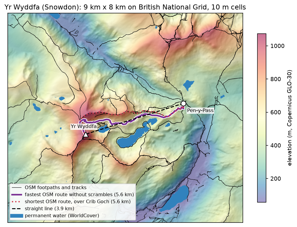
shortest_line = osm_route(G, "length", "shortest OSM route")
walkers = G.edge_subgraph([(a, b) for a, b, d in G.edges(data=True) if d["sac"] not in SCRAMBLES])
osm_line = osm_route(walkers, "minutes", "fastest OSM route without scrambles")

688 ways, 18936 nodes, 196.4 km of path in the box
sac_scale: (no sac_scale) 139.7 km, mountain_hiking 25.9 km, hiking 16.5 km, demanding_mountain_hiking 10.2 km, alpine_hiking 4.2 km
58 connected pieces; the largest holds 61% of the nodes
start snapped 128 m, end snapped 1 m to the path network
shortest OSM route: 5564 m, 171 min, 2480 m graded as scrambling | via Llwybr Llyn Llydaw 205 m, Craig Fach Track 711 m, (unnamed) 1076 m, Crib Goch 1378 m, (unnamed) 1609 m, Llanberis Path 513 m
fastest OSM route without scrambles: 5614 m, 132 min, 0 m graded as scrambling | via Llwybr Llyn Llydaw 205 m, Craig Fach Track 711 m, (unnamed) 280 m, Craig Fach Track 923 m, Llwybr Bwlch Moch 2578 m, Pyg Track 336 m, Llanberis Path 513 m

The shortest route goes over Crib Goch, a knife-edge ridge graded alpine_hiking that is a scramble, not a walk. The fastest route without scrambles follows Bwlch Moch and the Pyg Track, which is how most walkers from Pen-y-Pass climb the mountain. We call it the walkers’ route. The start point snapped 128 m to the path network. Every route below uses the same two snapped points, so the straight line is 3,920 m rather than 4,043 m.

Step 3: build the cost surface

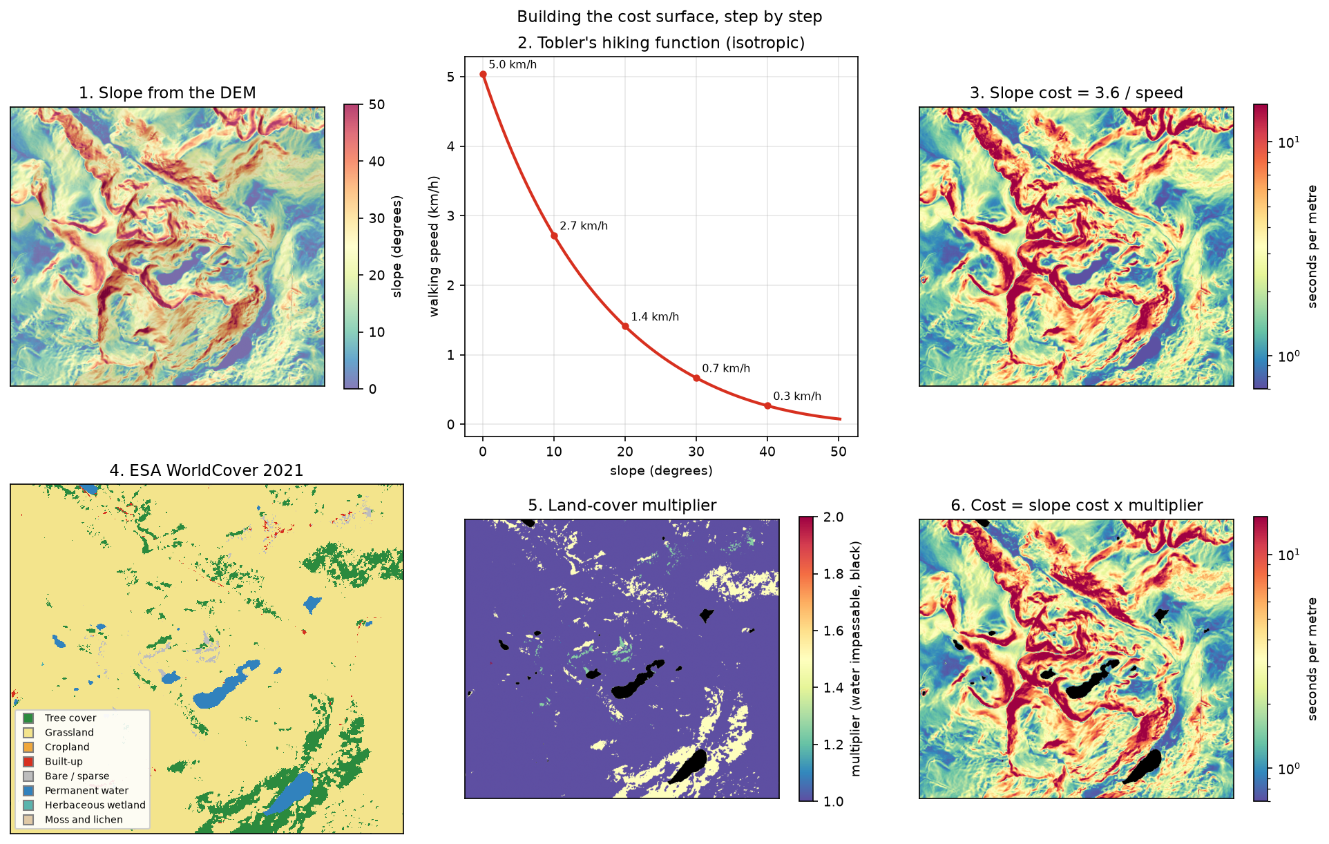
A cost surface turns everything that slows you down into one number per cell. For walking, a natural unit is seconds per metre. Start with slope from the DEM, then convert slope to speed with Tobler’s hiking function:

def tobler_kmh(s):
    """Tobler's hiking function. Pass a signed gradient for direction, or abs(gradient) for the isotropic form."""
    return 6.0 * np.exp(-3.5 * np.abs(s + 0.05))

gy, gx = np.gradient(dem, RES)
slope = np.hypot(gx, gy)                  # rise over run
slope_deg = np.degrees(np.arctan(slope))
speed = tobler_kmh(slope)                 # km/h; slope >= 0, so up and down cost the same
slope_cost = 3.6 / speed                  # seconds per metre

slope 18.6 deg median, 50.2 deg 99th percentile, 69.1 deg max
Tobler speed: 5.04 km/h on the flat, 1.41 km/h at 20 deg, 0.27 km/h at 40 deg

The 3.6 / speed converts km/h to seconds per metre: at 5 km/h a metre takes 0.72 s. Because slope is the steepest gradient in each cell, and is never negative, this cost is isotropic: crossing a cell costs the same in every direction. Step 7 removes that limitation.

Next, land cover. Each ESA WorldCover class gets a multiplier, and permanent water gets infinity, which makes it a barrier:

WC = {10: ("Tree cover", 1.5), 30: ("Grassland", 1.0), 40: ("Cropland", 1.2), 50: ("Built-up", 1.0),
      60: ("Bare / sparse", 1.25), 80: ("Permanent water", np.inf), 90: ("Herbaceous wetland", 2.0),
      100: ("Moss and lichen", 1.1)}          # the script also sets shrubland, snow and ice
lc_mult = np.ones_like(dem)
for code, (_, m) in WC.items():
    lc_mult[lc == code] = m
cost = slope_cost * lc_mult

   10 Tree cover             7.4% of cells  multiplier 1.5
   30 Grassland             90.0% of cells  multiplier 1.0
   40 Cropland               0.0% of cells  multiplier 1.2
   50 Built-up               0.3% of cells  multiplier 1.0
   60 Bare / sparse          0.5% of cells  multiplier 1.25
   80 Permanent water        1.8% of cells  multiplier inf
   90 Herbaceous wetland     0.0% of cells  multiplier 2.0
  100 Moss and lichen        0.0% of cells  multiplier 1.1
combined cost: 0.71-8028.15 s/m, 12932 impassable water cells

The multipliers are judgement, not measurement. They are typical of published walking models, but you should set your own for your terrain and your walkers. WorldCover labels 90% of this mountain as grassland, including much of the rocky ground, so here slope does nearly all the work.

Step 4: accumulated cost and the least-cost path

scikit-image’s MCP_Geometric (“minimum cost path”) does the rest. It treats the raster as a graph in which each cell connects to its eight neighbours. A move costs the mean of the two cells’ costs times the distance between their centres, so a diagonal step costs √2 times as much as a straight one. sampling=(RES, RES) sets the cell size, so costs per metre become seconds:

from skimage.graph import MCP_Geometric

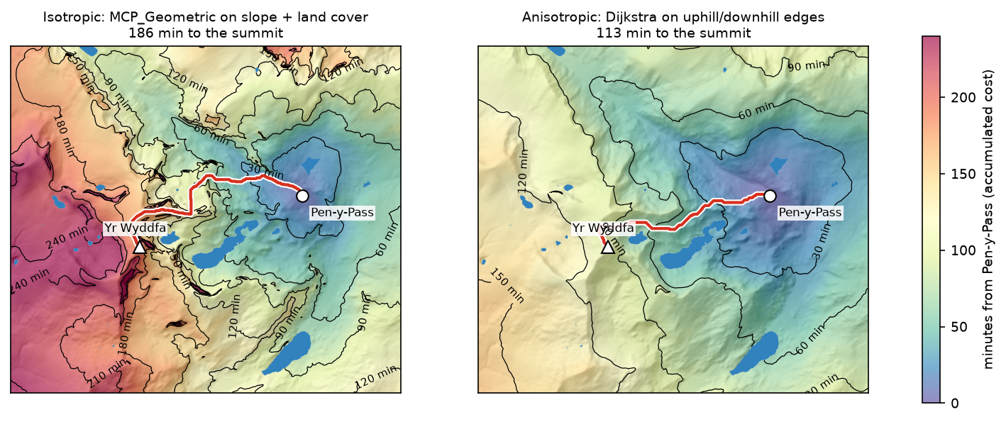
r0, c0 = rowcol(TRANSFORM, sx, sy)          # start cell (Pen-y-Pass)
r1, c1 = rowcol(TRANSFORM, ex, ey)          # end cell (the summit)
mcp = MCP_Geometric(cost, fully_connected=True, sampling=(RES, RES))
acc, _ = mcp.find_costs([(r0, c0)])         # accumulated cost from the start to every cell, in seconds
rc = np.array(mcp.traceback((r1, c1)))      # (row, col) of every cell on the least-cost path

MCP_Geometric on 720,000 cells: 0.15 s | accumulated cost at the summit 186 min
least-cost path: 5833 m, 516 cells | 12% within 50 m of the OSM route, 63% within 50 m of any mapped path, mean distance from the OSM route 503 m

find_costs computes the accumulated cost surface, the cost distance from Pen-y-Pass to all 720,000 cells, in 0.15 s. In travel-time units, its contours are isochrones. traceback follows it downhill from the summit back to the start. You can pass several start cells to find_costs (for example every cell of a road) to get the cost distance to the nearest of them.

Step 5: compare with the straight line and the footpaths

To compare routes fairly, the script walks each one uphill from Pen-y-Pass with the same rule. It samples the DEM every 10 m along the line, and applies Tobler’s function to the signed gradient along the route. It also reports Naismith’s rule, the ascent, the length over water, and how much of the route crosses terrain steeper than 30°:

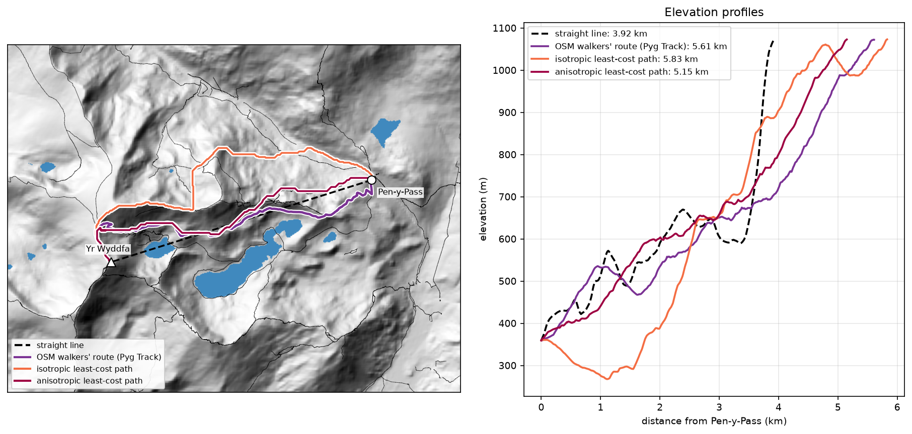
route                    length   Tobler  Naismith  ascent  water  >30 deg  steepest
straight line             3920m    676mn     141mn    938m   369m      32%      62deg
OSM walkers' route        5614m    124mn     149mn    815m     0m      19%      39deg
OSM shortest route        5564m    161mn     158mn    910m     0m      15%      50deg
least-cost path           5833m    154mn     160mn    903m     0m       5%      35deg

• The straight line is the shortest, but it crosses 369 m of Glaslyn, climbs terrain up to 62°, and takes 676 minutes by Tobler. Naismith’s rule gives a plausible 141 minutes only because it ignores steepness: it knows nothing about cliffs.
• The walkers’ route (Pyg Track) is the fastest at 124 minutes, with the least ascent (815 m). It is what the model should find.
• The isotropic least-cost path takes 154 minutes and keeps to gentle ground (only 5% over 30°). However, it drops north into the Llanberis Pass to 270 m before climbing, so 63% of it lies within 50 m of some mapped path but only 12% near the Pyg Track.

That last result shows the flaw of an isotropic cost. It charges each cell for its steepest gradient, whichever way you cross it. Walking along a contour on a 30° slope therefore costs as much as climbing straight up it, and losing height costs nothing extra. That is also why the accumulated cost at the summit (186 minutes) is longer than the same path walked with the signed gradient (154 minutes).

Step 6: how the cost weights change the route

A least-cost path is only as good as its cost surface. The script reruns MCP_Geometric with five versions of the cost, and walks each result with the same Tobler rule:

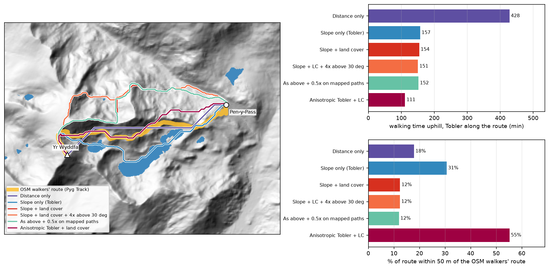
steep = np.where(slope_deg > 30, 4.0, 1.0)            # extra penalty for scrambling ground
scenarios = {
    "Distance only": np.where(lc == 80, np.inf, 1.0),
    "Slope only (Tobler)": slope_cost,
    "Slope + land cover": cost,
    "Slope + land cover + 4x above 30 deg": cost * steep,
    "As above + 0.5x on mapped paths": cost * steep * np.where(paths_mask == 1, 0.5, 1.0),
}

Distance only                          4229 m |  428 min | ascent  959 m | water    0 m |  56% over 30 deg |  18% within 50 m of the OSM route,  31% of any path | 0.12 s
Slope only (Tobler)                    5571 m |  157 min | ascent  845 m | water 1874 m |   6% over 30 deg |  31% within 50 m of the OSM route,  62% of any path | 0.15 s
Slope + land cover                     5833 m |  154 min | ascent  903 m | water    0 m |   5% over 30 deg |  12% within 50 m of the OSM route,  63% of any path | 0.14 s
Slope + land cover + 4x above 30 deg   5959 m |  151 min | ascent  908 m | water    0 m |   2% over 30 deg |  12% within 50 m of the OSM route,  43% of any path | 0.15 s
As above + 0.5x on mapped paths        6003 m |  152 min | ascent  904 m | water    0 m |   2% over 30 deg |  12% within 50 m of the OSM route,  77% of any path | 0.15 s
4-connected moves: 6600 m | 8-connected moves: 5833 m (diagonals cut the zigzag by 11.6%)

• Distance only, with water as the only barrier, gives the shortest possible dry route: 4.2 km, but 56% of it on ground steeper than 30°.
• Slope only walks 1.9 km straight across Llyn Llydaw. A lake is perfectly flat in a DEM, so to a slope-only model it is the best footpath on the mountain. This is the most common mistake in cost-surface building: every barrier the DEM cannot see must come from another layer.
• Adding land cover removes the lake but sends the route north, as in Step 5.
• A 4× penalty above 30° trims steep ground from 5% to 2% of the route.
• Halving the cost on mapped paths pulls 77% of the route onto paths, but onto the wrong ones. With an isotropic cost, the path bonus makes the model follow paths, not choose the right one.
• 4-connected moves make the route 11.6% longer than 8-connected moves, a reminder that raster routes are built from 45° and 90° steps.

Step 7: direction-aware (anisotropic) cost with SciPy

MCP_Geometric only accepts one cost per cell, so it cannot tell uphill from downhill. To get direction-aware costs, build the graph yourself. Every cell gets eight directed edges, one to each neighbour. Each edge’s cost is the time to walk that step at Tobler’s speed for the signed gradient along the step, times the mean land-cover multiplier of the two cells. NumPy slicing builds all 5.6 million edges at once:

from scipy import sparse
from scipy.sparse import csgraph

idx = np.arange(H * W).reshape(H, W)
src_l, dst_l, w_l = [], [], []
for dr, dc in [(-1, -1), (-1, 0), (-1, 1), (0, -1), (0, 1), (1, -1), (1, 0), (1, 1)]:
    rs = slice(max(0, -dr), H - max(0, dr)); cs_ = slice(max(0, -dc), W - max(0, dc))   # source cells
    rd = slice(rs.start + dr, rs.stop + dr); cd = slice(cs_.start + dc, cs_.stop + dc)     # their neighbours
    step_len = RES * np.hypot(dr, dc)
    grade = (dem[rd, cd] - dem[rs, cs_]) / step_len               # signed: positive is uphill
    secs = step_len * 3.6 / tobler_kmh(grade) * (lc_mult[rs, cs_] + lc_mult[rd, cd]) / 2
    ok = np.isfinite(secs)                                         # water edges are dropped
    src_l.append(idx[rs, cs_][ok]); dst_l.append(idx[rd, cd][ok]); w_l.append(secs[ok])
graph = sparse.csr_matrix((np.concatenate(w_l), (np.concatenate(src_l), np.concatenate(dst_l))),
                          shape=(H * W, H * W))
acc_aniso, pred = csgraph.dijkstra(graph, directed=True, indices=idx[r0, c0], return_predecessors=True)

The route comes from following pred back from the summit to the start, then converting the cell numbers back to rows and columns with np.unravel_index:

graph: 720,000 nodes, 5,641,358 directed edges, built in 0.25 s | Dijkstra 0.21 s
accumulated cost at the summit 113 min (isotropic: 186 min)
anisotropic least-cost path: 5153 m | Tobler 111 min | ascent 764 m | 32% over 30 deg | 55% within 50 m of the OSM route, 91% of any path | mean offset 102 m

This is the best model so far. The route is 5.15 km, 55% of it within 50 m of the Pyg Track and 91% within 50 m of a mapped path, with a mean offset from the Pyg Track of 102 m. It stays on the south side of the ridge, like the real path. It runs across steep slopes rather than straight up them, which is exactly what a zigzag footpath does. That is why 32% of its length crosses terrain steeper than 30°, while the gradient along the route stays walkable. Its ascent (764 m) is lower than the Pyg Track’s (815 m), because the mapped route loses and regains about 65 m between 1 and 2 km from Pen-y-Pass (Figure 4).

Pitfalls and limitations

• GLO-30 is a surface model at 30 m. Copernicus GLO-30 includes trees and buildings and is resampled here to 10 m, so it cannot see features of a few metres: path steps, boulder fields, small crags and the exact line of a zigzag. A bare-earth lidar DTM, resampled to a few metres, would sharpen the slope surface.
• Land cover is coarse and sometimes wrong. WorldCover classifies 90% of the box as grassland, including scree and rock. It also maps the Miners’ Track causeway across Llyn Llydaw as water, so that path is impassable in this cost surface. Barriers and passages under 10 m wide need vector data, rasterised onto the grid.
• Raster routes have a metric bias. Moves are restricted to 0°, 45° and 90°, so a route can be up to about 8% longer than the true shortest line on uniform ground, and it looks jagged. Step 6 shows the 4-connected versus 8-connected difference. Larger neighbourhoods (16 directions) or smoothing the result reduce the bias.
• Tobler’s function is a model of walking, not scrambling. It gives 0.27 km/h at 40°, but steeper ground is a question of skill and safety, not speed. A modelled route is not a safe route: never use one for navigation in place of a map and local guidance.
• One route is one answer. A least-cost path is the single optimum for one start, one end and one set of weights. Corridor analysis, which sums the accumulated cost from both ends, shows how much worse the nearly optimal alternatives are.
• Time from the cost surface. The isotropic accumulated cost (186 minutes) is not a travel time you should report, because it charges each cell for its steepest gradient. Walk the final line with a direction-aware rule, as in Step 5.

Frequently asked questions

What is least-cost path analysis?

Least-cost path analysis finds the route between two places that minimises a total cost rather than the distance. The cost can be time, energy, money or ecological resistance, and it is stored as a raster in which each cell holds the cost of crossing it. The algorithm first builds an accumulated cost surface from the start, then traces the cheapest route back from the destination. It is used for walking and hiking routes, pipelines and power lines, wildlife corridors and archaeology.

How do you calculate a least-cost path in Python?

Build a NumPy cost array, then use skimage.graph.MCP_Geometric(cost, sampling=(res, res)). Call find_costs([start_cell]) for the accumulated cost surface and traceback(end_cell) for the path as a list of (row, column) cells. Convert the cells to map coordinates with the raster’s affine transform. For direction-dependent costs, build a sparse directed graph of neighbouring cells and use scipy.sparse.csgraph.dijkstra, as in Step 7.

What is the difference between cost distance and least-cost path?

Cost distance (the accumulated cost surface) is a raster: for every cell it gives the lowest total cost of reaching it from the source. The least-cost path is a line: the single cheapest route to one destination, traced back through that surface. You compute the cost distance once and can trace paths to any number of destinations from it.

How do you make a cost surface from slope?

Compute slope from the DEM (for example with np.gradient), convert it to a speed or an effort with a function such as Tobler’s hiking function, and invert speed to time per metre. Then multiply by factors for land cover, roads or barriers, and set impassable cells to np.inf. Keep the units meaningful (seconds per metre here), so the accumulated cost is a travel time you can check.

Why does my least-cost path go through a lake?

Because the DEM shows the water surface as perfectly flat, so a slope-only cost makes the lake the cheapest ground in the area. Add a land-cover or water layer and set water cells to np.inf (or a very high cost), as in Step 6. The same applies to other barriers that a DEM cannot see, such as walls, fences, rivers and motorways.

Can QGIS or ArcGIS do the same thing?

Yes. ArcGIS Pro has Cost Distance, Cost Path and Distance Accumulation tools, and QGIS has the r.cost and r.walk tools from GRASS GIS, and plugins. r.walk is anisotropic and uses a Naismith-style walking model. Python gives you full control of the cost function and makes it easy to test many weightings, as in Step 6.

Next steps

• Compute slope, aspect and hillshade properly in DEM terrain analysis with rasterio, and see what you can see from the summit in viewshed analysis in Python.
• Route on a vector network instead of a raster with street networks in OSMnx, and turn travel times into service catchments with spatial accessibility (2SFCA).
• Replace WorldCover with your own land-cover map using random forest land-cover classification.
• Turn the route and the accumulated cost into an interactive map with Folium.
• Use the same DEM-to-graph thinking for water: height above nearest drainage (HAND) flood mapping routes flow over a DEM and measures how high each cell sits above its stream.

Data and licences

• DEM: Copernicus DEM GLO-30, © DLR e.V. 2010–2014 and © Airbus Defence and Space GmbH 2014–2018, provided under COPERNICUS by the European Union and ESA; all rights reserved, free to use under the Copernicus DEM licence. Accessed from the Microsoft Planetary Computer on 3 November 2026.
• Land cover: ESA WorldCover 10 m 2021 v200, © ESA WorldCover project 2021 / contains modified Copernicus Sentinel data (2021) processed by the ESA WorldCover consortium, licensed under CC BY 4.0. Accessed from the Microsoft Planetary Computer on 3 November 2026.
• Footpaths: © OpenStreetMap contributors, available under the Open Database Licence, queried through the Overpass API on 3 November 2026.
• Code: least_cost_path.py, tested with Python 3.12.0, scikit-image 0.26.0, numpy 2.5.4, scipy 1.18.1, networkx 3.7, rasterio 1.5.2, shapely 2.2.0 and pyproj 3.8.0.