Rapid situational mapping from open data in Python: the Valencia floods of 29 October 2024
Build a first situation map of a disaster from open data in Python. For the Valencia DANA floods of October 2024, read the Copernicus EMS activation and its first flood delineation, add municipalities, modelled rainfall from Open-Meteo and OpenStreetMap hospitals, schools, fire stations and bridges as they were on the morning of the flood, then make a one-page map, an interactive Folium map and a 'what we know' table.
- Level
- Beginner
- Tested with
- Python 3.12
- Source code
- Download scripts
Key takeaways
- A first situation map answers three questions: what happened, where, and what is in the way. Open data answers all three within hours to days: the Copernicus EMS activation, a modelled rainfall grid, municipal boundaries and OpenStreetMap facilities.
- Copernicus EMS was activated for Valencia 2 hours 10 minutes after the event time. The first flood delineation for L'Horta Sud arrived 84.2 hours after it, from WorldView-2 imagery of 31 October, and mapped 24.1 km² of flood extent.
- Most of that extent (23.23 km²) is flood trace, not standing water (0.84 km²). Two days after a flash flood, the water has gone and the mud remains, so read the notation field before you report a number.
- A 9 km weather model gives the pattern and timing of rain, not the peak. ECMWF IFS gives 127.8 mm at Turís on 29 October; the AEMET gauge there recorded 771 l/m² in 24 hours.
- Query OpenStreetMap as it was before the event with an Overpass attic date. Inside the mapped area, 24 of 208 schools, 2 of 54 health facilities, 1 of 39 fire and police stations and 88 of 288 road bridges were in the flood extent.
- Only count exposure inside the area that was actually mapped. Outside the EMS area of interest, 'no water' means 'not mapped', not 'dry'.
Before you start
- Basic Python and a first look at GeoPandas (reading files, plotting, spatial joins)
- Python 3.10+ with geopandas, osmnx, folium, matplotlib and requests
- An internet connection: the first run downloads about 61 MB from Copernicus EMS, geoBoundaries, Open-Meteo and the Overpass API and takes 3 to 10 minutes, depending on how busy the public Overpass server is
Short answer: a first situation map combines four kinds of open data that you can fetch from Python within hours of a disaster: the official event footprint (here the Copernicus EMS rapid mapping activation and its first flood delineation), administrative units (municipalities), the hazard driver (modelled rainfall) and what is exposed (hospitals, schools, emergency stations and bridges from OpenStreetMap, queried as they were before the event). Overlay them, count what falls inside the mapped flood extent, stamp the map with the time the information refers to, and summarise it in a short “what we know” table:
flood = read_ems("AOI03", "observedEventA") # Copernicus EMS first delineationfac["in_flood"] = fac.intersects(flood.union_all()) # OpenStreetMap facilities, as of 29 Octfac.groupby("facility")["in_flood"].agg(total="size", in_flood="sum")For the Valencia floods of 29 October 2024, the first Copernicus EMS delineation for L’Horta Sud mapped 24.1 km² of flood extent. Inside the mapped area, 24 of 208 schools, 2 of 54 health facilities and 88 of 288 road bridges were in it, and the worst-hit municipalities by area were Quart de Poblet, Riba-roja de Túria and Torrent.
On 29 October 2024 an isolated upper-level low, a DANA, stalled over eastern Spain. Rain of extraordinary intensity fell on the hills west of Valencia, and the Poyo ravine and other watercourses carried it as a flash flood into the dense towns of L’Horta Sud in the evening. The Spanish Government’s follow-up figures of 24 November 2024 record that more than 220 people died in the Comunitat Valenciana.
This is Part 1 of GIS for disaster emergency response, a six-part series that follows one event through the response lifecycle, written for GIS analysts who support civil protection, NGOs and local government. Part 1 builds the first situation map from open data. Part 2 maps the flood extent yourself from Sentinel-1 radar and Sentinel-2 optical imagery and measures how well it agrees with the Copernicus EMS product. Part 3 estimates the buildings and people exposed. Part 4 works out which roads, hospitals and neighbourhoods were cut off and where to put relief points. Part 5 builds a field survey for teams on the ground, and Part 6 packages the results for responders as files, a dashboard and a print-ready map.
You will learn how to:
- read a Copernicus EMS activation and its product timeline from the public API, and download a flood delineation as vector data;
- tell flood trace from flooded area, and a very high resolution delineation from a Sentinel-2 one;
- get municipal boundaries for Spain from geoBoundaries;
- pull modelled hourly rainfall for any point from the Open-Meteo archive, and know what it can and cannot tell you;
- query OpenStreetMap as it was before the event with an Overpass attic date, through OSMnx and directly;
- count facilities and bridges in the flood extent only where the extent was mapped;
- make a one-page situation map, an interactive Folium map and a “what we know” table with sources and times.
All outputs below are real results from situation_map.py, run on 17 November 2026 with Python 3.12, geopandas 1.2.0, osmnx 2.1.2 and folium 1.0.0.
What a first situation map is for
In the first hours of a disaster, responders need a shared picture: where the event is, which places are affected, and which hospitals, schools, stations and bridges are in the way. It does not need to be perfect. It needs to be sourced and dated, so everyone knows what each number means and how old it is.
Everything here is open and needs no account or key. The trade-off is time: each source arrives at its own pace, and the map is only as current as its oldest important layer. We will make that visible rather than hide it.
The study area is L’Horta Sud, from Torrent and Aldaia to the Albufera lagoon: longitude −0.60 to −0.30 and latitude 39.33 to 39.50, worked in ETRS89 / UTM zone 30N (EPSG:25830) for metres. It reaches 0.05° further west than a box drawn around the towns would, so that it holds the whole of the Copernicus EMS area for L’Horta Sud, including the Poyo ravine upstream of Torrent and Aldaia.
BBOX = (-0.60, 39.33, -0.30, 39.50) # lon/lat: L'Horta Sud, from Torrent and Aldaia to the AlbuferaCRS = "EPSG:25830" # ETRS89 / UTM zone 30N, metresACTIVATION = "EMSR773"EVENT_UTC = pd.Timestamp("2024-10-29 14:30", tz="UTC")OSM_DATE = "2024-10-29T00:00:00Z" # OpenStreetMap as it was on the morning of the floodRAIN_BOX = (-1.0, 39.1, -0.2, 39.7) # wider window: the rain fell upstream, in the Poyo catchmentStep 1: read the Copernicus EMS activation
The Copernicus Emergency Management Service (EMS) makes maps from satellite and aerial images for authorities dealing with a disaster. Spain activated it for Valencia as EMSR773. The rapid mapping portal has a public JSON API behind it, so one request returns the whole activation: its areas of interest (AOIs), every product, the sensor and image time, and when each product was delivered.
api = "https://rapidmapping.emergency.copernicus.eu/backend/dashboard-api/public-activations/"act = requests.get(api, params={"code": ACTIVATION}, headers=UA, timeout=60).json()["results"][0]print(f"{act['code']}: {act['name']} | {act['category']}, {len(act['aois'])} areas of interest")print(f"event {act['eventTime']} UTC, activated {act['activationTime']} UTC by {act['activator'].split('|')[0]}")
rows = []for aoi in act["aois"]: footprint = wkt.loads(aoi["extent"]) for p in aoi["products"]: img = p["images"][0] if p["images"] else {} rows.append({"aoi": f"AOI{aoi['number']:02d}", "name": aoi["name"], "type": p["type"], "monit": p.get("monitoringNumber") or 0, "sensor": img.get("sensorName"), "image_utc": pd.Timestamp(img.get("acquisitionTime"), tz="UTC"), "delivered_utc": pd.Timestamp(p["version"]["deliveryTime"], tz="UTC").floor("min"), "zip": p.get("downloadPath"), "in_study_area": footprint.intersects(box(*BBOX))})products = pd.DataFrame(rows)products["hours_after_event"] = ((products.delivered_utc - EVENT_UTC).dt.total_seconds() / 3600).round(1)local = products[products.in_study_area].sort_values("delivered_utc")EMSR773: Flood in Valencia Region, Spain | Flood, 36 areas of interestevent 2024-10-29T14:30:00 UTC, activated 2024-10-29T16:40:00 UTC by Spain44 products in total; 12 cover the study area: aoi name type monit sensor image_utc delivered_utc hours_after_eventAOI03 Horta Sud DEL 0 WorldView-2 2024-10-31 10:22:00+00:00 2024-11-02 02:43:00+00:00 84.2AOI01 Valencia province DEL 0 Sentinel-2 2024-10-31 10:51:00+00:00 2024-11-02 03:02:00+00:00 84.5AOI01 Valencia province DEL 1 ICEYE 2024-11-03 01:51:00+00:00 2024-11-03 18:18:00+00:00 123.8AOI03 Horta Sud GRA 0 GeoEye-1 2024-10-31 10:22:00+00:00 2024-11-06 03:36:00+00:00 181.1AOI01 Valencia province DEL 2 Sentinel-2 2024-11-05 10:52:00+00:00 2024-11-06 07:08:00+00:00 184.6AOI01 Valencia province DEL 3 Sentinel-1 2024-11-06 06:00:00+00:00 2024-11-06 13:10:00+00:00 190.7AOI01 Valencia province DEL 4 COSMO-SkyMed Second Generation 2024-11-08 05:51:00+00:00 2024-11-08 10:55:00+00:00 236.4AOI13 Monserrat GRA 0 Pleiades 2024-11-10 10:39:00+00:00 2024-11-11 23:54:00+00:00 321.4AOI20 Montroi GRA 0 Plane Imagery 2024-11-11 10:00:00+00:00 2024-11-16 05:10:00+00:00 422.7AOI30 Valencia Sud GRA 0 Plane Imagery 2024-11-17 13:21:00+00:00 2024-11-16 11:11:00+00:00 428.7AOI35 Alcasser GRA 0 Plane Imagery 2024-11-17 13:21:00+00:00 2024-11-27 13:12:00+00:00 694.7AOI36 Paterna GRA 0 Plane Imagery 2024-11-18 12:16:00+00:00 2024-11-29 09:46:00+00:00 739.3The table is a timeline of what an analyst could know and when. The activation came 2 hours 10 minutes after the event time. The first flood outline for L’Horta Sud came 84.2 hours after it, from a WorldView-2 image taken on the morning of 31 October and delivered early on 2 November. Damage grading (GRA) followed four days later. Until 2 November, a situation map of this area could only show where the rain fell and what was there, not where the water went. That gap is why Part 2 of this series maps flood extent directly from free satellite data.
Step 2: read the first flood delineation
Each product is a zip of shapefiles. The flood polygons are in the layer ending _observedEventA, and the footprint that was mapped is in _areaOfInterestA. GeoPandas reads straight from the zip, so a small helper downloads the product once and returns any layer in metres:
first = local[(local.type == "DEL") & (local.monit == 0)].set_index("aoi")

def read_ems(aoi: str, layer: str) -> gpd.GeoDataFrame:    url = first.loc[aoi, "zip"]    path = get(url, DATA / Path(url).name)    name = next(n for n in zipfile.ZipFile(path).namelist() if n.endswith(f"_{layer}_v1.shp"))    return gpd.read_file(f"zip://{path.as_posix()}!{name}").to_crs(CRS)

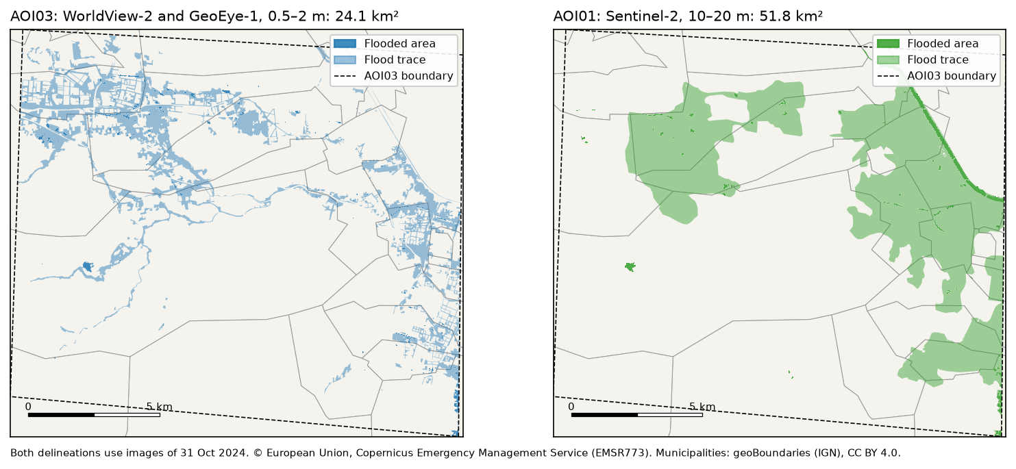
flood = read_ems("AOI03", "observedEventA")aoi03 = read_ems("AOI03", "areaOfInterestA")s2 = gpd.clip(read_ems("AOI01", "observedEventA"), aoi03)flood["km2"] = flood.area / 1e6print(flood.groupby(["notation", "det_method"])["km2"].agg(["count", "sum"]).round(2).to_string())AOI03 Horta Sud: 242 km² mapped from WorldView-2 imagery of 31 Oct 2024 10:22 UTC count sumnotation det_methodFlood trace Photo-interpretation 311 23.23Flooded area Semi-automatic extraction 306 0.84observed flood extent (flooded area + flood trace): 24.1 km²same area in the AOI01 Sentinel-2 delineation: 51.8 km²Read the notation column before you report a number. Only 0.84 km² was standing water when the image was taken. The other 23.23 km² is flood trace: streets, fields and yards the water had reached and left, marked by mud and debris and picked out by an analyst. A flash flood drains within hours, and the first clear image came almost two days later. For a picture of where the flood went, the trace is what you want, so the rest of this tutorial uses both classes together as the “observed flood extent”.
The province-wide Sentinel-2 delineation, clipped to the same footprint, gives 51.8 km², more than twice as much. Sentinel-2 pixels are 10 to 20 m, against about 0.5 m for WorldView-2, so its polygons are broad blobs that swallow streets and blocks, while the very high resolution product follows the streets themselves. Neither is “the truth”; they answer the question at different scales. Part 2 compares flood maps like these properly, with an agreement matrix.
Step 3: add municipalities
Responders organise by municipality, so every number needs a municipality next to it. geoBoundaries publishes Spain’s municipal boundaries (ADM3, from the national mapping agency IGN) as one GeoJSON under CC BY 4.0. We pin a specific commit so the file does not change under us, read only the window we need with bbox=, and record how much of each municipality lies inside AOI03, because that is the only part we can say anything about:
gb = get("https://github.com/wmgeolab/geoBoundaries/raw/9469f09/releaseData/gbOpen/ESP/ADM3/" "geoBoundaries-ESP-ADM3_simplified.geojson", DATA / "geoBoundaries-ESP-ADM3_simplified.geojson")muni_all = gpd.read_file(gb, bbox=RAIN_BOX).to_crs(CRS)[["shapeName", "geometry"]]muni_all = muni_all.rename(columns={"shapeName": "municipality"})muni = muni_all[muni_all.intersects(study.geometry[0])].copy()muni["mapped_km2"] = muni.intersection(aoi03.union_all()).area / 1e6 # area the EMS mapped133 municipalities in the rainfall window, 33 touch the study areaStep 4: add rainfall for 29 October
Most of the water that flooded L’Horta Sud fell upstream, in the hills drained by the Poyo ravine. To show that, we need rainfall over a wider window than the study area. Two things matter in the first hours: where the rain fell and when.
The Open-Meteo historical weather API serves hourly archives of several models, with no key, under CC BY 4.0. We ask for the ECMWF IFS model at 9 km on a 0.1° grid of 63 points, and for hourly rain at three places: Chiva and Turís in the hills where the rain fell, and Paiporta on the plain where the Poyo ravine broke through. For comparison, we also ask for the coarser ERA5 reanalysis at about 25 km.
ARCHIVE = "https://archive-api.open-meteo.com/v1/archive"lons = np.round(np.arange(RAIN_BOX[0], RAIN_BOX[2] + 0.01, 0.1), 2)lats = np.round(np.arange(RAIN_BOX[1], RAIN_BOX[3] + 0.01, 0.1), 2)LON, LAT = np.meshgrid(lons, lats)grid = requests.get(ARCHIVE, headers=UA, timeout=120, params={    "latitude": ",".join(map(str, LAT.ravel())), "longitude": ",".join(map(str, LON.ravel())),    "start_date": "2024-10-29", "end_date": "2024-10-29", "daily": "precipitation_sum",    "models": "ecmwf_ifs", "timezone": "Europe/Madrid"}).json()rain = np.array([g["daily"]["precipitation_sum"][0] for g in grid]).reshape(LAT.shape)
pts = requests.get(ARCHIVE, headers=UA, timeout=120, params={ "latitude": ",".join(str(v[1]) for v in PLACES.values()), "longitude": ",".join(str(v[0]) for v in PLACES.values()), "start_date": "2024-10-29", "end_date": "2024-10-30", "hourly": "precipitation", "daily": "precipitation_sum", "models": "ecmwf_ifs,era5", "timezone": "Europe/Madrid"}).json()63 grid points, 0.1° spacing; 29 Oct total 28-193 mm, maximum at -0.9°, 39.1°Chiva IFS 114.2 mm | ERA5 87.2 mm | wettest hour 19:00 local, 13.7 mmTurís IFS 127.8 mm | ERA5 87.2 mm | wettest hour 18:00 local, 18.2 mmPaiporta IFS 111.5 mm | ERA5 66.6 mm | wettest hour 13:00 local, 16.4 mm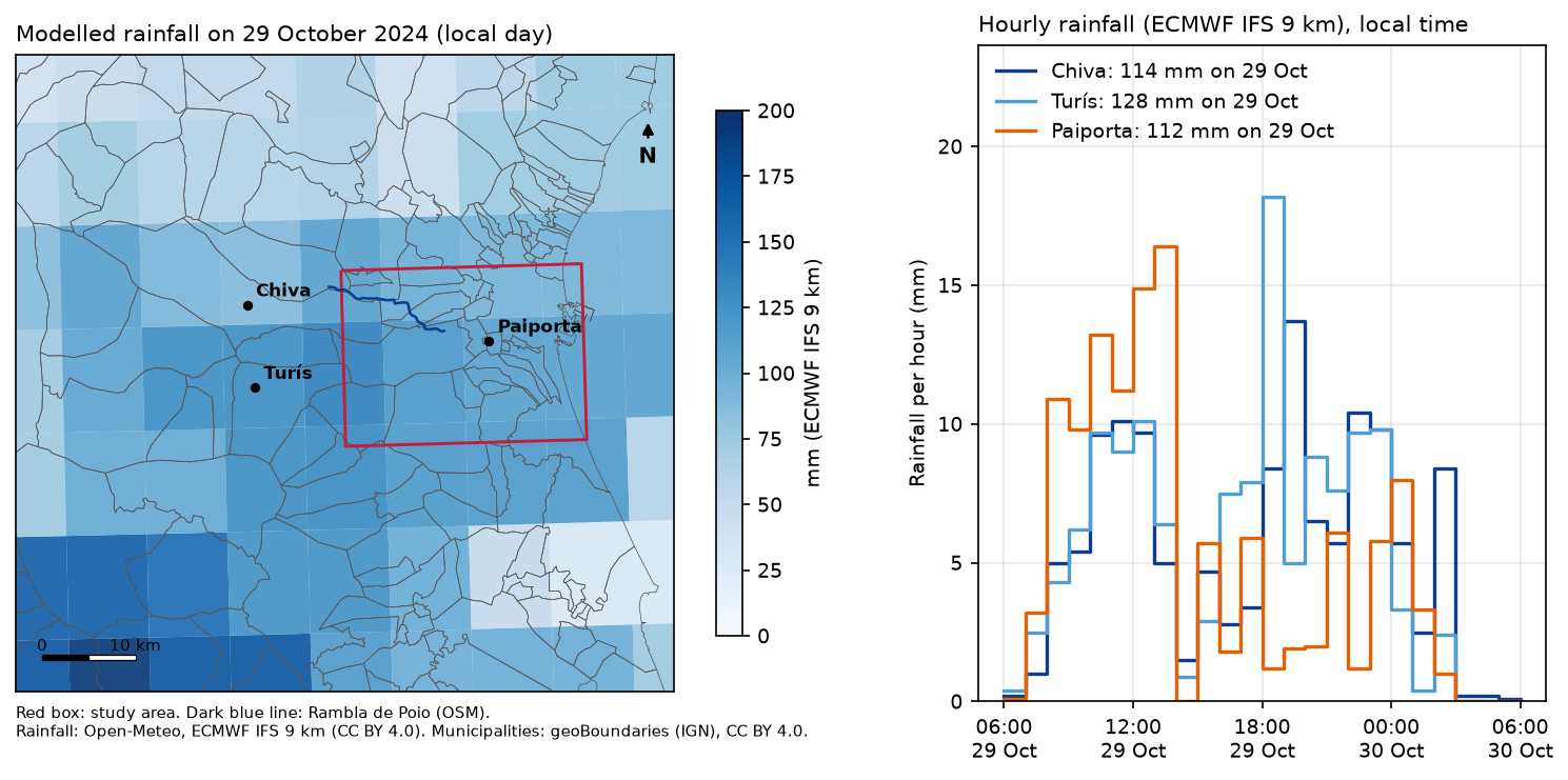
The pattern is right: the heaviest rain fell inland, west and south-west of the towns that flooded, and the hills had their wettest hours in the early evening. The amounts are not. The AEMET weather station at Turís recorded 771 l/m² in 24 hours, 185 of them in a single hour, a Spanish record for one hour. The model gives 127.8 mm for the whole day there, and its wettest hour is 18.2 mm. A 9 km grid cell averages the rain over 81 km², so a storm only a few kilometres across is smeared out; ERA5, at about 25 km, smooths it even more.
Step 5: get critical facilities from OpenStreetMap, as they were on the morning of the flood
OpenStreetMap is the richest open source of hospitals, schools, emergency stations and bridges, and after a disaster volunteers edit it intensively. That is good for the response, but it means today’s data is not what the map looked like on the day. The Overpass API can answer attic queries: add a [date:...] setting and it returns the data as it was at that moment. OSMnx passes it through if you set it in overpass_settings:
ox.settings.use_cache = Trueox.settings.cache_folder = str(DATA / "osm_cache")ox.settings.requests_timeout = 300ox.settings.overpass_settings = f'[out:json][timeout:{{timeout}}][date:"{OSM_DATE}"]{{maxsize}}'
fac = osm({"amenity": ["hospital", "clinic", "school", "fire_station", "police"],           "healthcare": ["hospital", "centre"], "emergency": ["ambulance_station"]}).reset_index()
# "facility", not "type": GeoDataFrame.type is a built-in property that returns geometry typesfac["facility"] = fac.apply(facility_type, axis=1)
Here osm() wraps ox.features.features_from_bbox with a polite retry, because the public Overpass server is often busy, and facility_type() turns the tags into six readable classes. Name the column facility, not type: GeoDataFrame.type already exists and returns the geometry type, so fac.type would quietly give you “Point” and “Polygon”.
For roads, bridges, railways and rivers we send one raw Overpass query and ask for way geometries directly with out tags geom. It is lighter on the server than asking OSMnx for every feature that carries any of these tags. A road bridge is any vehicle road way tagged bridge=yes or bridge=viaduct:
VEHICLE = "motorway|trunk|primary|secondary|tertiary|unclassified|residential|living_street|service"s, w, n, e = BBOX[1], BBOX[0], BBOX[3], BBOX[2]query = f"""[out:json][timeout:600][date:"{OSM_DATE}"];(way["highway"~"^(motorway|trunk|primary|secondary)(_link)?$"]({s},{w},{n},{e}); way["bridge"~"^(yes|viaduct)$"]["highway"~"^({VEHICLE})(_link)?$"]({s},{w},{n},{e}); way["railway"="rail"]({s},{w},{n},{e}); way["waterway"~"^(river|canal|stream)$"]({s},{w},{n},{e}););out tags geom;"""r = requests.post("https://overpass-api.de/api/interpreter", data={"data": query}, headers=UA, timeout=700)571 facilities in the study area: School 376, Health centre 100, Police 57, Hospital 24, Fire station 11, Ambulance station 33769 major road ways, 572 rail ways, 391 waterways, 487 road bridgesPoyo ravine in OSM: Rambla de Poio, 1 way, 15.3 km in the study areaThe last line is a small lesson in itself. On the morning of the flood, OpenStreetMap named only one way of the Poyo ravine, as “Rambla de Poio”, 15.3 km from Riba-roja to Picanya. Downstream, through Paiporta, the channel had no name. A search for “Poyo” alone would have missed it, and a search by name finds nothing in the town where the flood was worst. Check names in both local languages (Valencian Poio, Spanish Poyo) and look at the geometry, not just the attributes.
Step 6: what is in the flood?
Now the overlay. One rule matters more than any other: only count inside the area that was mapped. AOI03 covers 242 km². Outside it, a school with no flood polygon around it is not “dry”; nobody looked. So we keep only the facilities and bridges inside AOI03, then test each against the dissolved flood extent:
# Only the area inside AOI03 was mapped. Outside it, "no water" means "not mapped", not "dry".mapped = aoi03.union_all()fac = fac[fac.intersects(mapped)].copy()bridges = bridges[bridges.intersects(mapped)].copy()extent = flood.dissolve()[["geometry"]]fac["in_flood"] = fac.intersects(extent.geometry[0])bridges["in_flood"] = bridges.intersects(extent.geometry[0])bridges["over_poyo"] = bridges.intersects(poyo.union_all().buffer(5))fac = gpd.sjoin(fac, muni[["municipality", "geometry"]], how="left", predicate="intersects") \    .drop_duplicates(["element", "id"]).drop(columns="index_right")
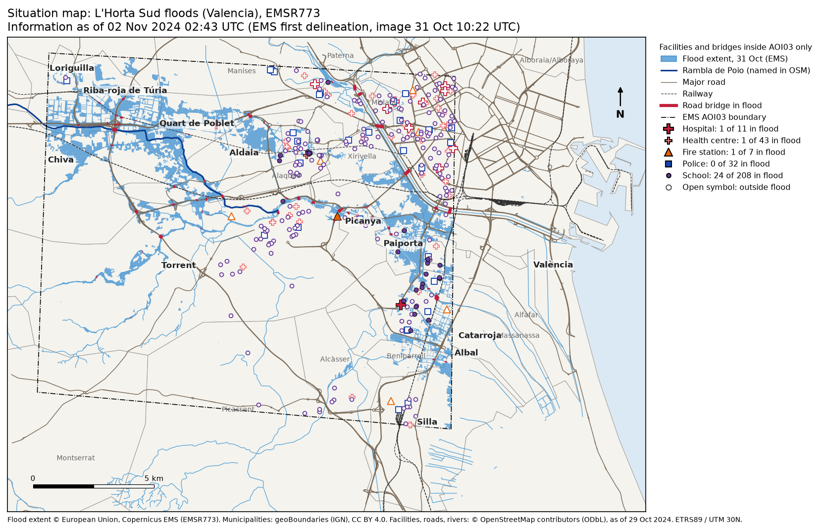
by_type = fac.groupby("facility")["in_flood"].agg(total="size", in_flood="sum")inside AOI03: 301 facilities and 288 road bridges total in_floodfacilitySchool 208 24Health centre 43 1Police 32 0Hospital 11 1Fire station 7 1road bridges in the flood extent: 88 of 288; road bridges over the Poyo ravine: 11
Facilities inside the flood extent (excluding schools): facility name municipality Fire station Parc de Bombers de Torrent TorrentHealth centre Centre de Salut d'Alaquàs Alaquàs Hospital (no name in OSM) CatarrojaFacilities are points or building outlines, so intersects counts a school whose grounds touch the flood extent, not only one whose centre is under water. That suits a first screening: it errs towards including places someone should check. The ambulance stations in the study area all lie outside AOI03, so they drop out of the table. The hospital in Catarroja has no name in OpenStreetMap; in a real response, that is the kind of gap you would fix in OSM or note on the map.
Then the same counts per municipality. mapped_km2 is the part of each municipality inside AOI03, and flood_pct is the share of that part in the flood extent:
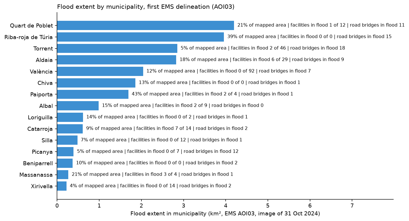
fl_muni = gpd.overlay(flood[["geometry"]], muni[["municipality", "geometry"]], how="intersection")summary = muni.set_index("municipality")[["mapped_km2"]].copy()fl_muni["km2"] = fl_muni.area / 1e6summary["flood_km2"] = fl_muni.groupby("municipality")["km2"].sum()summary["facilities"] = fac.groupby("municipality").size()summary["facilities_in_flood"] = fac[fac.in_flood].groupby("municipality").size()summary["bridges_in_flood"] = bridges[bridges.in_flood].groupby("municipality").size()summary = summary.fillna(0)summary["flood_pct"] = 100 * summary.flood_km2 / summary.mapped_km2summary = summary[summary.flood_km2 >= 0.05].sort_values("flood_km2", ascending=False)20 municipalities with at least 5 ha in the flood extent (flood_pct = share of the mapped part): mapped_km2 flood_km2 facilities facilities_in_flood bridges_in_flood flood_pctmunicipalityQuart de Poblet 19.7 4.20 12 1 11 21.3Riba-roja de Túria 10.2 3.96 0 0 15 38.8Torrent 62.9 2.85 46 2 18 4.5Aldaia 15.9 2.83 29 6 9 17.7València 17.1 2.04 92 0 7 11.9Chiva 14.0 1.86 0 0 1 13.3Paiporta 3.9 1.69 4 2 1 43.3Albal 6.6 0.99 9 2 0 14.9Loriguilla 4.3 0.61 2 0 1 14.4Catarroja 6.7 0.61 14 7 2 9.1Silla 7.1 0.48 12 0 1 6.8Picanya 7.3 0.39 7 0 12 5.4Beniparrell 3.6 0.37 0 0 2 10.3Massanassa 1.2 0.27 4 3 1 21.5Xirivella 5.2 0.22 14 0 2 4.3Alfafar 0.9 0.21 3 2 0 22.6Alcàsser 9.0 0.13 5 0 0 1.4Alaquàs 3.8 0.13 18 1 5 3.3Manises 7.9 0.12 7 0 0 1.5Benetússer 0.8 0.06 5 1 0 8.0Area and impact rank differently. Quart de Poblet and Riba-roja de Túria top the list by area. Paiporta has only 1.69 km² in the extent, but that is 43.3% of its mapped area, and it is dense housing. Catarroja has 7 facilities in the flood extent, the most of any municipality, and Picanya has 12 road bridges in it, where the ravine runs through the town. A situation map should show all three views: area, share and what is exposed.
Step 7: write the “what we know” table
The last analysis step turns all of this into eight lines that someone can read out at a coordination meeting. Every line has a source and an as of time, because the layers are not equally fresh: the facilities are from the morning of 29 October, the flood extent from an image of 31 October, and the product was delivered on 2 November.
know = pd.DataFrame([ ("Event", f"Extraordinary rainfall from {EVENT_UTC:%d %b %Y %H:%M} UTC", "Copernicus EMS EMSR773", f"{pd.Timestamp(act['activationTime']):%d %b %H:%M} UTC"), ("Flood extent", f"{flood.km2.sum():.1f} km² in L'Horta Sud", "EMS AOI03 first delineation", f"image {aoi03_row.image_utc:%d %b %H:%M} UTC"), ("Road bridges", f"{bridges.in_flood.sum()} in the flood extent, {bridges.over_poyo.sum()} over the Poyo ravine", "OSM + EMS", "OSM 29 Oct"), # ... rainfall, municipalities, health facilities, schools and emergency services in the full script], columns=["topic", "what we know", "source", "as of"])know.to_csv(OUT / "what_we_know.csv", index=False) topic what we know source as of Event Extraordinary rainfall from 29 Oct 2024 14:30 UTC Copernicus EMS EMSR773 29 Oct 16:40 UTC Rainfall, 29 Oct up to 193 mm (ECMWF IFS 9 km, max of 63 grid points); Chiva 114 mm, Paiporta 112 mm Open-Meteo 29 Oct (local day) Flood extent 24.1 km² in L'Horta Sud EMS AOI03 first delineation image 31 Oct 10:22 UTC Municipalities 20 with ≥5 ha flooded; most: Quart de Poblet, Riba-roja de Túria, Torrent geoBoundaries + EMS 02 Nov 02:43 UTC Health facilities 2 of 54 in the flood extent OSM + EMS OSM 29 Oct Schools 24 of 208 in the flood extent OSM + EMS OSM 29 OctEmergency services 1 of 39 stations in the flood extent OSM + EMS OSM 29 Oct Road bridges 88 in the flood extent, 11 over the Poyo ravine OSM + EMS OSM 29 Octwrote situation_emsr773.gpkg (4 layers) and what_we_know.csvThe script also writes the flood extent, facilities, bridges and municipalities to one GeoPackage, situation_emsr773.gpkg, so the next analyst can open the same layers in QGIS or ArcGIS Pro without rerunning anything.
The one-page situation map
The map puts everything on one page in a fixed order, from background to foreground: municipalities, the flood extent, rivers and the Poyo ravine, major roads and railways, the AOI03 boundary, road bridges in the flood, and then the facilities. A filled symbol is a facility in the flood extent; an open one is outside it. The title carries the “information as of” time, the delivery time of the flood product, and the credit line names every source. The legend counts are the ones from Step 6, so the map and the table can never disagree.
Step 8: an interactive map
A static map is what goes into a briefing, but analysts and coordinators want to zoom in and click. Folium writes a single HTML file with the same layers, a tooltip on every facility and bridge, and a layer switcher. Schools are switched off at first, because 208 purple dots hide everything else:
m = folium.Map(location=[centre.y, centre.x], zoom_start=12, tiles="OpenStreetMap", control_scale=True)web = flood[["notation", "geometry"]].copy()web["geometry"] = web.simplify(3)folium.GeoJson(web.to_crs(4326), name="Flood extent, 31 Oct (Copernicus EMS)", style_function=lambda f: {"color": "#1f5fa8", "weight": 0, "fillColor": "#3d8fd1", "fillOpacity": 0.6 if f["properties"]["notation"] == "Flooded area" else 0.35}, tooltip=folium.GeoJsonTooltip(["notation"], labels=False)).add_to(m)for t, (_, c, _) in STYLE.items(): layer = folium.FeatureGroup(name=f"{t} (OSM)", show=t != "School") # one CircleMarker per facility: larger with a black outline when it is in the flood extent layer.add_to(m)folium.LayerControl(collapsed=False).add_to(m)html = OUT / "situation_map.html"m.save(html)wrote situation_map.html: 1.43 MBSimplifying the flood polygons by 3 m keeps their shape and the file small enough to share by email or a messaging app.
Limitations and how to improve them
- The flood extent is days old. It shows where water had been by 31 October, not the peak on the evening of 29 October; later monitoring products and Part 2’s satellite methods add to it.
- Modelled rain underestimates the peak by a factor of about six at Turís; add AEMET station data or radar for amounts.
- OpenStreetMap completeness varies. Some facilities are missing or unnamed; check the key ones against official registers such as the regional health and education directories.
- Intersects is generous. A large school site touching the extent counts as in it; for building-level exposure, Part 3 uses building footprints.
Frequently asked questions
How quickly does Copernicus EMS deliver maps after a disaster?
It depends first on getting a usable image: satellite passes, cloud and the size of the area all add time before mapping can start. For EMSR773 the activation came 2 hours 10 minutes after the event time; the first usable image of L’Horta Sud was taken on 31 October, and its delineation was delivered 84.2 hours after the event. Read the timeline from the API, as in Step 1, so you know what exists for your area and when.
What is the difference between flooded area and flood trace?
Flooded area is standing water visible in the image. Flood trace is land the water reached but had left by the time of the image, recognised by mud, debris and wet surfaces. In the first AOI03 delineation, 0.84 km² was flooded area and 23.23 km² was flood trace.
Who can activate Copernicus EMS, and can anyone download the data?
Activations are requested by authorised users, mainly national civil protection authorities and EU bodies. The products are free for anyone to download and reuse under the Copernicus EMS terms, with the source credited.
Why query OpenStreetMap as it was before the event?
After a disaster, volunteers map damage, closures and new facilities quickly. That helps the response, but the current data then mixes the pre-event state with changes caused by the event. An Overpass attic date such as [date:"2024-10-29T00:00:00Z"] gives you a consistent baseline of what was there before.
Can I use ERA5 or Open-Meteo rainfall to say how much rain fell?
Use them for where and when it rained, not for peak amounts. In this case the ECMWF IFS 9 km archive gave 127.8 mm at Turís on 29 October and ERA5 gave 87.2 mm, while the AEMET station there recorded 771 l/m² in 24 hours. Gridded data averages rain over whole cells, so small, intense storms are smoothed out.
Can I run this for another disaster?
Yes. Change the activation code, the bounding box, the event time, the OSM date and the rainfall window in the settings block. The EMS API, Open-Meteo, Overpass and geoBoundaries all work worldwide; only the layer names inside EMS products and the facility tags may need a check.
Next steps
- Map flood extent from free radar yourself, with no wait for a rapid mapping product, in Sentinel-1 SAR flood mapping in Python.
- Build drivable road networks from OpenStreetMap, the basis of the routing in Part 4, in Street networks with OSMnx.
- Style and share richer web maps in Interactive web maps with Folium.
- Find the land most likely to flood before the next event with height above nearest drainage (HAND) in Python.
- For an earthquake rather than a flood, see earthquake damage mapping with Sentinel-1.
Data and licences
- Copernicus EMS rapid mapping, activation EMSR773: product timeline and the first delineation products for AOI03 (Horta Sud) and AOI01 (Valencia province), from the rapid mapping portal and its public API, accessed on 17 November 2026. © European Union, Copernicus Emergency Management Service. Free, full and open access under Regulation (EU) 2021/696 and the Copernicus EMS terms and conditions.
- Municipalities: geoBoundaries, Spain ADM3, simplified, from data of the Instituto Geográfico Nacional (IGN), via GitHub at commit 9469f09, accessed on 17 November 2026. Licensed CC BY 4.0. Runfola, D. et al. (2020), “geoBoundaries: A global database of political administrative boundaries”, PLoS ONE 15(4): e0231866.
- Rainfall: ECMWF IFS 9 km and ERA5 archives from the Open-Meteo historical weather API, accessed on 17 November 2026. Weather data by Open-Meteo.com, licensed CC BY 4.0; contains modified Copernicus Climate Change Service information (ERA5) and ECMWF data.
- Station rainfall quoted for comparison: Agencia Estatal de Meteorología (AEMET), October 2024 climate summary and report on the DANA episode of 29 October 2024.
- Facilities, roads, bridges, railways and rivers: © OpenStreetMap contributors, available under the Open Database Licence, as of 29 October 2024 00:00 UTC, through the Overpass API (overpass-api.de) and OSMnx, accessed on 17 November 2026. Map tiles in the interactive map © OpenStreetMap contributors.
- Casualty figures: Government of Spain, La Moncloa, DANA follow-up data, 24 November 2024.
- Code:
situation_map.py, tested with Python 3.12.0, geopandas 1.2.0, osmnx 2.1.2, folium 1.0.0, matplotlib 3.11.2, pandas 3.1.1, numpy 2.5.5, shapely 2.2.0, pyproj 3.8.0, pyogrio 0.13.0 and requests 2.34.2.
Key terms
- DANA
- Depresión aislada en niveles altos, an isolated upper-level low (a cut-off low). A pool of cold air aloft, cut off from the main jet stream, that can sit over warm Mediterranean water and fuel slow-moving, extremely heavy rain in autumn.
- Copernicus EMS Rapid Mapping
- The on-demand mapping component of the Copernicus Emergency Management Service. An authorised user, usually a national civil protection authority, activates it, and it delivers satellite-based maps and vector data within hours to days, free of charge.
- Activation
- A request to Copernicus EMS for one event, with a code such as EMSR773. It holds one or more areas of interest, each with its own products.
- Area of interest (AOI)
- The footprint that one Copernicus EMS product covers. Data outside it was not mapped, which is different from data showing no flooding.
- Delineation (DEL)
- A Copernicus EMS product that outlines the extent of the event, here the flood, from one satellite or aerial image. Monitoring products repeat it with later images.
- Grading (GRA)
- A Copernicus EMS product that assesses the damage to buildings, roads and other assets, usually from very high resolution imagery.
- Flood trace
- Land the water reached but has since left, recognised by mud, debris and wet surfaces. Copernicus EMS maps it separately from flooded area, which is standing water at the time of the image.
- Overpass attic query
- An Overpass API query with a date setting, such as [date:"2024-10-29T00:00:00Z"], that returns OpenStreetMap as it was at that moment, before any edits made after the event.
- Situation map
- A map that shows the current known state of an emergency for the people responding to it, with the time the information refers to and its sources.
Data for this tutorial
- Copernicus Emergency Management Service, rapid mapping · Activation EMSR773: timeline and the first flood delineations for AOI03 (Horta Sud) and AOI01 (Valencia province)
- geoBoundaries · Spain ADM3 (municipalities), simplified, from IGN data
- OpenStreetMap · Hospitals, health centres, schools, fire and police stations, roads, bridges, railways and rivers as of 29 October 2024, via the Overpass API
- ERA5 · ERA5 reanalysis rainfall, compared with the ECMWF IFS 9 km archive through the Open-Meteo historical weather API
Licences and formats for each source are listed in the GIS data sources catalogue.


